Overview
The strollur package stores data associated with your Amplicon Sequence Analysis. This tutorial will familiarize you with some of the functions available in the strollur package. If you haven’t reviewed the “Getting Started” tuturial, we recommend you start there.
Loading the example dataset
We can use the miseq_sop_example() function to create a
dataset object from the Miseq SOP Example.
miseq <- miseq_sop_example()
#> Added 2425 sequences.
#> Assigned 2425 sequence abundances.
#> Assigned 2425 sequence taxonomies.
#> Assigned 531 otu bins.
#> Assigned 2425 asv bins.
#> Assigned 63 phylotype bins.
#> Assigned 19 samples to treatments.
#> Assigned 531 otu bin taxonomies.
#> Assigned 531 otu bin representative sequences.
#> Added a metadata report.
#> Added 2 resource references.
#> Added a contigs_report report.
To print a summary of the miseq dataset, run the following:
miseq
#> miseq_sop:
#>
#>             starts ends nbases ambigs polymers numns   numseqs
#> Minimum:         1  375    249      0        3     0      1.00
#> 2.5%-tile:       1  375    252      0        4     0   2849.08
#> 25%-tile:        1  375    252      0        4     0  28490.75
#> Median:          1  375    253      0        4     0  56981.50
#> 75%-tile:        1  375    253      0        5     0  85472.25
#> 97.5%-tile:      1  375    254      0        6     0 111113.93
#> Maximum:         1  375    256      0        6     0 113963.00
#> Mean:            1  375    252      0        4     0  56981.64
#>
#> Number of unique seqs: 2425
#> Total number of seqs: 113963
#>
#> Total number of samples: 19
#> Total number of treatments: 2
#> Total number of otus: 531
#> Total number of otu bin classifications: 531
#> Total number of asvs: 2425
#> Total number of asv bin classifications: 2425
#> Total number of phylotypes: 63
#> Total number of phylotype bin classifications: 63
#> Total number of sequence classifications: 2425
#> Total number of resource references: 2
#> Total number of custom reports: 2
Accessing Your Data
The strollur package includes several functions to access your sequence data.
names() - The names function is an extension of base R’s
names function. It allows you to get the name of your dataset or the
names of the sequences, bins, samples, treatments and reports in your
dataset.
count() - The count function allows you to get the
number of sequences, bins, samples and treatments in your dataset.
abundance() - The abundance function can be used to
access the abundance data for sequences, bins, samples, and
treatments.
report() - The report function can be used to access the
various data associated with your dataset.
summary() - The summary function allows you to summarize
sequences, your custom reports, and scrapped data.
names
The names() function allows you to get the names of
sequences, bins, samples, treatments and reports. Let’s take a closer
look at how use it.
To get the name of the dataset, set the type parameter to ‘dataset’:
names(miseq, type = "dataset")
#> [1] "miseq_sop"
To get the names of the sequences in your dataset, set the type parameter to ‘sequence’:
all_sequences <- names(
  miseq,
  type = "sequence",
  distinct = FALSE
)
length(all_sequences)
#> [1] 2425
head(all_sequences, n = 5)
#> [1] "M00967_43_000000000-A3JHG_1_2101_16474_12783"
#> [2] "M00967_43_000000000-A3JHG_1_1113_12711_3318"
#> [3] "M00967_43_000000000-A3JHG_1_2108_14707_9807"
#> [4] "M00967_43_000000000-A3JHG_1_1110_4126_16552"
#> [5] "M00967_43_000000000-A3JHG_1_2102_8408_13436"
To get the names of the sequences present in sample ‘F3D0’:
include_f3d0 <- names(
  miseq,
  type = "sequence",
  samples = c("F3D0"),
  distinct = FALSE
)
length(include_f3d0)
#> [1] 309
head(include_f3d0, n = 5)
#> [1] "M00967_43_000000000-A3JHG_1_2103_25452_6018"
#> [2] "M00967_43_000000000-A3JHG_1_1109_13330_21597"
#> [3] "M00967_43_000000000-A3JHG_1_1110_5315_13833"
#> [4] "M00967_43_000000000-A3JHG_1_2104_26311_10309"
#> [5] "M00967_43_000000000-A3JHG_1_1101_9620_19745"
To get the names of the sequences exclusive to sample ‘F3D0’:
exclusive_f3d0 <- names(
  miseq,
  type = "sequence",
  samples = c("F3D0"),
  distinct = TRUE
)
length(exclusive_f3d0)
#> [1] 101
head(exclusive_f3d0, n = 5)
#> [1] "M00967_43_000000000-A3JHG_1_2103_25452_6018"
#> [2] "M00967_43_000000000-A3JHG_1_1101_9620_19745"
#> [3] "M00967_43_000000000-A3JHG_1_2109_17345_6668"
#> [4] "M00967_43_000000000-A3JHG_1_1114_14431_2336"
#> [5] "M00967_43_000000000-A3JHG_1_2106_14305_11884"
To get the names of the bins in your dataset, you need to specify the bin_type. The miseq example contains 3 bin types: otu, asv and phylotype. Let’s find the bin names for the ‘otu’ bin type.
otu_bins <- names(
  miseq,
  type = "bin",
  bin_type = "otu"
)
length(otu_bins)
#> [1] 531
head(otu_bins, n = 5)
#> [1] "Otu001" "Otu002" "Otu003" "Otu004" "Otu005"
To get the names of the ‘otu’ bins that include sequences present in sample ‘F3D0’:
include_f3d0 <- names(
  miseq,
  type = "bin",
  samples = c("F3D0"),
  distinct = FALSE
)
length(include_f3d0)
#> [1] 191
head(include_f3d0, n = 5)
#> [1] "Otu001" "Otu002" "Otu003" "Otu004" "Otu005"
To get the names of the “otu” bins that are exclusive to sample ‘F3D0’:
exclusive_f3d0 <- names(
  miseq,
  type = "bin",
  samples = c("F3D0"),
  distinct = TRUE
)
length(exclusive_f3d0)
#> [1] 14
head(exclusive_f3d0, n = 5)
#> [1] "Otu330" "Otu339" "Otu341" "Otu345" "Otu347"
To get the names of the samples
names(miseq, type = "sample")
#>  [1] "F3D0"   "F3D1"   "F3D141" "F3D142" "F3D143" "F3D144" "F3D145" "F3D146"
#>  [9] "F3D147" "F3D148" "F3D149" "F3D150" "F3D2"   "F3D3"   "F3D5"   "F3D6"
#> [17] "F3D7"   "F3D8"   "F3D9"
To get the names of the treatments
names(miseq, type = "treatment")
#> [1] "Early" "Late"
To get the names of the custom reports
names(miseq, type = "report")
#> [1] "contigs_report" "metadata"
count
The count() function allows you to get the number of
sequences, bins, samples and treatments in your dataset.
To find the total number of sequences in the dataset, run the following:
count(
  miseq,
  type = "sequence",
  distinct = FALSE
)
#> [1] 113963
To find the number of unique sequences in the dataset, set ‘distinct’ to TRUE:
count(
  miseq,
  type = "sequence",
  distinct = TRUE
)
#> [1] 2425
To get total number of sequences present in sample ‘F3D0’, you can set the samples parameter. Note, these sequences will be present in the sample but may be be present in other samples as well.
To get number of unique sequences exclusive to sample ‘F3D0’:
To get the number of the bins in your dataset, you need to specify the bin_type. The miseq example contains 3 bin types: otu, asv and phylotype. Let’s find the number of bins for the ‘otu’ bin type.
count(
  miseq,
  type = "bin",
  bin_type = "otu"
)
#> [1] 531
To get number of otu bins with sequences present in sample ‘F3D0’: Note these bins will have sequences from sample ‘F3D0’ and may contain sequences from other samples as well.
To get number of otu bins exclusive to sample ‘F3D0’: Note these bins will have sequences from sample ‘F3D0’ and NO other samples will be present in the bins.
To get the number of samples in the dataset:
count(miseq, type = "sample")
#> [1] 19
To get the number of treatments in the dataset:
count(miseq, type = "treatment")
#> [1] 2
abundance
Now that we are familiar with the names() and
count() functions. Let’s learn how we can use the
abundance() function. The abundance function can be used to
access the abundance data for sequences, bins, samples, and treatments.
It returns a data.frame containing the requested abundance data.
To the total abundance for each sequence, set the type = ‘sequence’. This will return a 2 column data.frame containing sequence_names and abundances.
sequence_abundance <- abundance(
  miseq,
  type = "sequence",
  by_sample = FALSE
)
head(sequence_abundance, n = 10)
#>                                   sequence_name abundance
#> 1  M00967_43_000000000-A3JHG_1_2101_16474_12783         1
#> 2   M00967_43_000000000-A3JHG_1_1113_12711_3318         1
#> 3   M00967_43_000000000-A3JHG_1_2108_14707_9807         1
#> 4   M00967_43_000000000-A3JHG_1_1110_4126_16552         1
#> 5   M00967_43_000000000-A3JHG_1_2102_8408_13436         1
#> 6  M00967_43_000000000-A3JHG_1_1107_22580_21773         1
#> 7  M00967_43_000000000-A3JHG_1_1108_14299_17220       191
#> 8   M00967_43_000000000-A3JHG_1_1114_8059_18290         1
#> 9    M00967_43_000000000-A3JHG_1_2112_9811_9982         1
#> 10  M00967_43_000000000-A3JHG_1_2103_25452_6018         1
To the abundance for each sequence parsed by sample, set by_sample = TRUE. This will return a 3 or 4 column data.frame containing sequence_names, abundances, samples and treatments (if assigned).
sequence_abundance_by_sample <- abundance(
  miseq,
  type = "sequence",
  by_sample = TRUE
)
head(sequence_abundance_by_sample, n = 10)
#>                                   sequence_name abundance sample treatment
#> 1  M00967_43_000000000-A3JHG_1_2101_16474_12783         1 F3D150      Late
#> 2   M00967_43_000000000-A3JHG_1_1113_12711_3318         1 F3D142      Late
#> 3   M00967_43_000000000-A3JHG_1_2108_14707_9807         1   F3D3     Early
#> 4   M00967_43_000000000-A3JHG_1_1110_4126_16552         1   F3D8     Early
#> 5   M00967_43_000000000-A3JHG_1_2102_8408_13436         1   F3D7     Early
#> 6  M00967_43_000000000-A3JHG_1_1107_22580_21773         1   F3D3     Early
#> 7  M00967_43_000000000-A3JHG_1_1108_14299_17220        22 F3D146      Late
#> 8  M00967_43_000000000-A3JHG_1_1108_14299_17220        19 F3D147      Late
#> 9  M00967_43_000000000-A3JHG_1_1108_14299_17220        12 F3D148      Late
#> 10 M00967_43_000000000-A3JHG_1_1108_14299_17220         9 F3D149      Late
To get the total abundance of the bins in your dataset, you need to specify the bin_type. The miseq example contains 3 bin types: otu, asv and phylotype. Let’s find the abundance data of bins for the otu bin type. This will return a 2 column data.frame containing bin_names and abundances.
bin_abundance <- abundance(
  miseq,
  type = "bin",
  bin_type = "otu",
  by_sample = FALSE
)
head(bin_abundance, n = 10)
#>    otu_id abundance
#> 1  Otu001     12288
#> 2  Otu002      8892
#> 3  Otu003      7794
#> 4  Otu004      7476
#> 5  Otu005      7450
#> 6  Otu006      6621
#> 7  Otu007      6304
#> 8  Otu008      5337
#> 9  Otu009      3606
#> 10 Otu010      3061
To the abundance for each bin parsed by sample, set by_sample = TRUE. This will return a 3 or 4 column data.frame containing bin_names, abundances, samples and treatments (if assigned).
bin_abundance_by_sample <- abundance(
  miseq,
  type = "bin",
  bin_type = "otu",
  by_sample = TRUE
)
head(bin_abundance_by_sample, n = 10)
#>    bin_name abundance sample treatment
#> 1    Otu001       499   F3D0     Early
#> 2    Otu001       351   F3D1     Early
#> 3    Otu001       388 F3D141      Late
#> 4    Otu001       244 F3D142      Late
#> 5    Otu001       189 F3D143      Late
#> 6    Otu001       346 F3D144      Late
#> 7    Otu001       566 F3D145      Late
#> 8    Otu001       270 F3D146      Late
#> 9    Otu001      1316 F3D147      Late
#> 10   Otu001       750 F3D148      Late
To access the distribution of sequences across the samples in your dataset, set the type = ‘sample’. This will return a 2 column data.frame containing sample names and abundances.
abundance(
  miseq,
  type = "sample"
)
#>    sample abundance
#> 1    F3D0      6191
#> 2    F3D1      4652
#> 3  F3D141      4656
#> 4  F3D142      2423
#> 5  F3D143      2403
#> 6  F3D144      3449
#> 7  F3D145      5532
#> 8  F3D146      3831
#> 9  F3D147     12430
#> 10 F3D148      9465
#> 11 F3D149     10014
#> 12 F3D150      4126
#> 13   F3D2     15686
#> 14   F3D3      5199
#> 15   F3D5      3469
#> 16   F3D6      6394
#> 17   F3D7      4055
#> 18   F3D8      4253
#> 19   F3D9      5735
To access the distribution of sequences across the treatments in your dataset, set the type = ‘treatment’. This will return a 2 column data.frame containing treatment names and abundances.
abundance(miseq, type = "treatment")
#>   treatment abundance
#> 1     Early     55634
#> 2      Late     58329
report
The report() function allows you access you to access
FASTA sequences, sequence and classification reports, bin assignments,
sample assignments, metadata, sequence data reports, custom reports,
resource references and scrapped data reports. It returns a data.frame
containing the requested report data. Let’s look at some examples
together.
To get a report containing the sequences FASTA data, set the type = “fasta”. This will be a 2 or 3 column data.frame containing sequence names, sequence nucleotide strings, and comments (if provided).
fasta_report <- report(
  miseq,
  type = "fasta"
)
head(fasta_report, n = 5)
#>                                  sequence_name
#> 1 M00967_43_000000000-A3JHG_1_2101_16474_12783
#> 2  M00967_43_000000000-A3JHG_1_1113_12711_3318
#> 3  M00967_43_000000000-A3JHG_1_2108_14707_9807
#> 4  M00967_43_000000000-A3JHG_1_1110_4126_16552
#> 5  M00967_43_000000000-A3JHG_1_2102_8408_13436
#>                                                                                                                                                                                                                                                                                                                                                                                  sequence
#> 1 TAC--GG-AG-GAT--GCG-A-G-C-G-T-T--AT-C-CGTGAT--TT-A-T-T--GG-GT--TT-A-AA-GG-GT-GC-G-TA-GGC-G-G-A-CA-G-T-T-AA-G-T-C-A-G-C-G-G--TA-A-AA-TT-G-A-GA-GG--CT-C-AA-C-C-T-C-T-T-C--CC-G-C-CGTT-GAAAC-TG-A-TTGTC-TTGA-GT-GG-GC-GA-G-A---AG-T-A-TGTGGAATGCGTGGTGT-AGCGGT-GAAATGCATAG-AT-A-TC-AC-GC-AG-AACTCCGAT-TGCGAAGGCA------GCATA-CCG-G-CG-CC-C-A-ACTGACG-CTGA-AGCA-CGAAA-GCG-TGGGT-ATC-GAACAGG
#> 2 TAC--GT-AG-GGG--GCA-A-G-C-G-T-T--AT-C-CGG-AT--TT-A-C-T--GG-GT--GT-A-AA-GG-GA-GC-G-TA-GGC-G-G-C-CA-T-G-C-AA-G-T-C-A-G-A-A-G--TG-A-AA-AC-C-C-GG-GG--CT-C-AA-C---C-C-TGG-G-AGT-G-C-TTTT-GAAAC-TG-T-GCGGC-TAGA-GT-GT-CG-GA-G-G---GG-T-A-AGTGGAATTCCTAGTGT-AGCGGT-GAAATGCGTAG-AT-A-TT-AG-GA-GG-AACACCAGT-GGCGAAGGCG------GCTTA-CTG-G-AC-GA-T-G-ACTGACG-CTGA-GGCT-CGAAA-GCG-TGGGT-ATC-GAACAGG
#> 3 TAC--GG-AG-GAT--GCG-A-G-C-G-T-T--AT-C-CGG-AT--TT-A-C-T--GG-GT--GT-A-AA-GG-GA-GC-G-TA-GAC-G-G-C-GG-C-G-C-AA-G-T-C-T-G-A-A-G--TG-A-AA-GC-C-C-GT-GG--CT-C-AA-C-C-G-C-G-G-A-ACC-G-C-TTTG-GAAAC-TG-C-GAGGC-TGGA-GT-GC-TG-GA-G-A---GG-T-A-AGCGGAATTCCTGGTGT-AGCGGT-GAAATGCGTAG-AT-A-TC-AG-GA-GG-AACACCGGT-GGCGAAGGCG------GCTTA-CTG-G-AC-AG-T-G-ACTGACG-TTGA-GGCT-CGAAA-GCG-TGGGG-AGC-GAACAGG
#> 4 TAC--GG-AG-GAT--TCA-A-G-C-G-T-T--AT-C-CGG-AT--TT-A-T-T--GG-GT--TT-A-AA-GG-GT-GC-G-TA-GGC-G-G-G-CT-G-T-T-AA-G-T-C-A-G-C-G-G--TC-A-AA-TG-T-C-GG-GG--CT-C-AA-C-C-C-C-G-G-C--CT-G-C-CGTT-GAAAC-TG-G-CGGCC-TCGA-GT-GG-GC-GA-G-A---AG-T-A-TGCGGAATGCGTGGTGT-AGCGGT-GAAATGCATAG-AT-A-TC-AC-GC-AG-AACTCCGAT-TGCGAAGGCA------GCATA-CCG-G-CG-CC-C-T-ACTGACG-CTGA-GGCA-CGAAA-GCG-TGGGT-ATC-GAACAGG
#> 5 TAC--GG-AG-GGG--GCA-A-G-C-G-T-T--AT-C-CGG-AT--TT-A-C-T--GG-GT--GT-A-AA-GG-GA-GC-G-TA-GGC-G-G-C-AG-T-G-C-AA-G-T-C-A-G-A-A-G--TG-A-AA-GC-C-C-AA-GG--CT-C-AA-C---C-A-TGG-G-ACT-G-C-TTTT-GAAAC-TG-T-ACAGC-TAGA-TT-GC-AG-GA-G-A---GG-T-A-AGTGGAATTCCTAGTGT-AGCGGT-GAAATGCGTAG-AT-A-TT-AG-GA-GG-AACACCAGT-GGCGAAGGCG------GCTTA-CTG-G-AC-TG-T-A-AATGACG-CTGA-GGCT-CGAAA-GCG-TGGGG-AGC-AAACAGG
If you want to take a closer look at the sequences, you can request a report containing the sequence names, starts, ends, lengths, ambiguous bases, longest homopolymers, and number of N’s. To get a sequence report, set type = “sequence”.
sequence_report <- report(
  miseq,
  type = "sequence"
)
head(sequence_report, n = 5)
#>                                  sequence_name start end length ambig
#> 1 M00967_43_000000000-A3JHG_1_2101_16474_12783     1 375    253     0
#> 2  M00967_43_000000000-A3JHG_1_1113_12711_3318     1 375    253     0
#> 3  M00967_43_000000000-A3JHG_1_2108_14707_9807     1 375    253     0
#> 4  M00967_43_000000000-A3JHG_1_1110_4126_16552     1 375    252     0
#> 5  M00967_43_000000000-A3JHG_1_2102_8408_13436     1 375    253     0
#>   longest_homopolymer num_n
#> 1                   4     0
#> 2                   5     0
#> 3                   4     0
#> 4                   4     0
#> 5                   5     0
The report function also allows you to access classification reports about your dataset. There are 2 types of classification reports: sequence_taxonomy and bin_taxonomy. To get a report about the sequence classifications, set type = “sequence_taxonomy”. This will create a 3 or 4 column report containing sequence names, taxonomic levels, taxons and confidence scores(if provided).
sequence_classification <- report(
  miseq,
  type = "sequence_taxonomy"
)
head(sequence_classification, n = 10)
#>                                   sequence_name level
#> 1  M00967_43_000000000-A3JHG_1_2101_16474_12783     1
#> 2  M00967_43_000000000-A3JHG_1_2101_16474_12783     2
#> 3  M00967_43_000000000-A3JHG_1_2101_16474_12783     3
#> 4  M00967_43_000000000-A3JHG_1_2101_16474_12783     4
#> 5  M00967_43_000000000-A3JHG_1_2101_16474_12783     5
#> 6  M00967_43_000000000-A3JHG_1_2101_16474_12783     6
#> 7   M00967_43_000000000-A3JHG_1_1113_12711_3318     1
#> 8   M00967_43_000000000-A3JHG_1_1113_12711_3318     2
#> 9   M00967_43_000000000-A3JHG_1_1113_12711_3318     3
#> 10  M00967_43_000000000-A3JHG_1_1113_12711_3318     4
#>                             taxonomy confidence
#> 1                           Bacteria        100
#> 2                    "Bacteroidetes"        100
#> 3                      "Bacteroidia"         99
#> 4                    "Bacteroidales"         99
#> 5               "Porphyromonadaceae"         88
#> 6  "Porphyromonadaceae"_unclassified         88
#> 7                           Bacteria        100
#> 8                         Firmicutes        100
#> 9                         Clostridia        100
#> 10                     Clostridiales        100
To get the consensus taxonomies assigned to the bins in your dataset, you need to specify the bin_type. The miseq example contains 3 bin types: otu, asv and phylotype. Let’s find the consensus taxonomies of bins for the otu bin type.
bin_classification <- report(
  miseq,
  type = "bin_taxonomy",
  bin_type = "otu"
)
head(bin_classification, n = 10)
#>    bin_name level                          taxonomy confidence
#> 1    Otu001     1                          Bacteria        100
#> 2    Otu001     2                   "Bacteroidetes"        100
#> 3    Otu001     3                     "Bacteroidia"        100
#> 4    Otu001     4                   "Bacteroidales"        100
#> 5    Otu001     5              "Porphyromonadaceae"        100
#> 6    Otu001     6 "Porphyromonadaceae"_unclassified        100
#> 7    Otu002     1                          Bacteria        100
#> 8    Otu002     2                   "Bacteroidetes"        100
#> 9    Otu002     3                     "Bacteroidia"        100
#> 10   Otu002     4                   "Bacteroidales"        100
To get the sequence bin assignments for the otu bins, run the following:
sequence_bin_assignments <- report(
  miseq,
  type = "sequence_bin_assignment",
  bin_type = "otu"
)
head(sequence_bin_assignments, n = 10)
#>    otu_id                                       seq_id
#> 1  Otu001  M00967_43_000000000-A3JHG_1_1111_20933_6700
#> 2  Otu001  M00967_43_000000000-A3JHG_1_1113_17095_9759
#> 3  Otu001 M00967_43_000000000-A3JHG_1_1114_22144_24942
#> 4  Otu001   M00967_43_000000000-A3JHG_1_1112_5981_8948
#> 5  Otu001  M00967_43_000000000-A3JHG_1_2106_5509_18056
#> 6  Otu001 M00967_43_000000000-A3JHG_1_1112_18411_17052
#> 7  Otu001 M00967_43_000000000-A3JHG_1_1101_20262_22075
#> 8  Otu001 M00967_43_000000000-A3JHG_1_1114_13556_18457
#> 9  Otu001 M00967_43_000000000-A3JHG_1_2114_12634_10967
#> 10 Otu001 M00967_43_000000000-A3JHG_1_1102_18640_14309
To get the sample treatment assignments, set type = “sample_assignment”.
sample_treatment_assignments <- report(
  miseq,
  type = "sample_assignment"
)
head(sample_treatment_assignments, n = 5)
#>   sample treatment
#> 1   F3D0     Early
#> 2   F3D1     Early
#> 3 F3D141      Late
#> 4 F3D142      Late
#> 5 F3D143      Late
If you assigned bin representative sequences, you can access the report by setting type = “bin_representative”. The miseq example includes bin representatives for the otu bins. Let’s take a look:
otu_bin_representatives <- report(
  miseq,
  type = "bin_representative",
  bin_type = "otu"
)
head(otu_bin_representatives, n = 5)
#>   otu_names                          representative_name
#> 1    Otu001 M00967_43_000000000-A3JHG_1_1108_14299_17220
#> 2    Otu002  M00967_43_000000000-A3JHG_1_1106_22705_6123
#> 3    Otu003  M00967_43_000000000-A3JHG_1_1101_15533_5293
#> 4    Otu004 M00967_43_000000000-A3JHG_1_1105_25642_17588
#> 5    Otu005  M00967_43_000000000-A3JHG_1_2102_7041_13746
#>                                                                                                                                                                                                                                                                                                                                                                   representative_sequence
#> 1 TAC--GT-AG-GGG--GCA-A-G-C-G-T-T--AT-C-CGG-AT--TT-A-C-T--GG-GT--GT-A-AA-GG-GA-GC-G-TA-GAC-G-G-C-TG-T-G-C-AA-G-T-C-T-G-A-A-G--TG-A-AA-TG-C-C-GG-GG--CT-C-AA-C-C-C-C-G-G-A-ACT-G-C-TTTG-GAAAC-TG-T-ACAGC-TAGA-GT-GC-AG-GA-G-G---GG-T-G-AGCGGAATTCCTAGTGT-AGCGGT-GAAATGCGTAG-AT-A-TT-AG-GA-GG-AACACCGGT-GGCGAAGGCG------GCTCA-CTG-G-AC-TG-T-A-ACTGACG-TTGA-GGCT-CGAAA-GCG-TGGGG-AGC-AAACAGG
#> 2 TAC--GT-AG-GGG--GCA-A-G-C-G-T-T--AT-C-CGG-AT--TT-A-C-T--GG-GT--GT-A-AA-GG-GA-GC-G-CA-GAC-G-G-C-TG-T-G-C-AA-G-T-C-T-G-G-A-G--TG-A-AA-GG-C-G-GG-GG--CC-C-AA-C-C-C-C-C-G-G-ACT-G-C-TCTG-GAAAC-TG-T-AAAGC-TGGA-GT-GC-AG-GA-G-A---GG-T-A-AGCGGAATTCCTAGTGT-AGCGGT-GAAATGCGTAG-AT-A-TT-AG-GA-GG-AACACCAGT-GGCGAAGGCG------GCTTA-CTG-G-AC-TG-C-A-ACTGACG-TTGA-GGCT-CGAAA-GCG-TGGGT-ATC-GAACAGG
#> 3 TAC--GG-AG-GAT--GCG-A-G-C-G-T-T--AT-C-CGG-AT--TT-A-C-T--GG-GT--GT-A-AA-GG-GA-GC-G-TA-GAC-G-G-C-GA-T-G-C-AA-G-T-C-T-G-A-A-G--TG-A-AA-GG-C-G-GG-GG--CC-C-AA-C-C-C-C-C-G-G-ACT-G-C-TTTG-GAAAC-TG-T-ATAGC-TGGA-GT-GC-AG-GA-G-A---GG-T-A-AGTGGAATTCCTAGTGT-AGCGGT-GAAATGCGTAG-AT-A-TT-AG-GA-GG-AACACCAGT-GGCGAAGGCG------GCTTA-CTG-G-AC-TG-T-A-ACTGACG-TTGA-GGCT-CGAAA-GCG-TGGGG-AGC-AAACAGG
#> 4 TAC--GT-AG-GTG--GCA-A-G-C-G-T-T--AT-C-CGG-AT--TT-A-C-T--GG-GT--GT-A-AA-GG-GC-GT-G-TA-GGC-G-G-G-AC-T-G-C-AA-G-T-C-A-G-A-T-G--TG-A-AA-CC-C-A-TG-GG--CT-C-AA-C-C-C-A-T-G-G-CCT-G-C-ATTT-GAAAC-TG-T-AGTTC-TTGA-GT-GA-TG-GA-G-A---GG-C-A-GGCGGAATTCCGTGTGT-AGCGGT-GAAATGCGTAG-AT-A-TA-CG-GA-GG-AACACCAGT-GGCGAAGGCG------GCCTG-CTG-G-AC-AT-T-A-ACTGACG-CTGA-GGCG-CGAAA-GCG-TGGGG-AGC-AAACAGG
#> 5 TAC--GT-AG-GGG--GCG-A-G-C-G-T-T--AT-C-CGG-AT--TC-A-T-T--GG-GC--GT-A-AA-GC-GC-GC-G-CA-GGC-G-G-A-CT-C-A-T-AA-G-C-G-G-A-G-C-C--TT-T-AA-TC-T-T-GG-GG--CT-T-AA-C-C-T-C-A-A-G-T-C-G-G-GCCC-CGAAC-TG-T-GAGTC-TCGA-GT-GT-GG-TA-G-G---GG-A-A-GGCGGAATTCCCGGTGT-AGCGGT-GGAATGCGCAG-AT-A-TC-GG-GA-AG-AACACCGAT-GGCGAAGGCA------GCCTT-CTG-G-GC-CA-T-C-ACTGACG-CTGA-GGCG-CGAAA-GCT-AGGGG-AGC-AAACAGG
The miseq example contains a custum report. To access the custom reports, first let’s find the names.
names(miseq, type = "report")
#> [1] "contigs_report" "metadata"
To access the custom contigs assembly report, set type = “contigs_report”.
contigs_assembly_report <- report(
  miseq,
  type = "contigs_report"
)
head(contigs_assembly_report, n = 5)
#>                                           Name Length Overlap_Length
#> 1 M00967_43_000000000-A3JHG_1_2101_16474_12783    253            250
#> 2  M00967_43_000000000-A3JHG_1_1113_12711_3318    253            249
#> 3  M00967_43_000000000-A3JHG_1_2108_14707_9807    253            249
#> 4  M00967_43_000000000-A3JHG_1_1110_4126_16552    252            249
#> 5  M00967_43_000000000-A3JHG_1_2102_8408_13436    253            249
#>   Overlap_Start Overlap_End MisMatches Num_Ns Expected_Errors
#> 1             2         252         19      0      0.29461400
#> 2             2         251          0      0      0.00183396
#> 3             2         251          0      0      0.00196774
#> 4             2         251          4      0      0.05629750
#> 5             2         251          0      0      0.00259554
To get the metadata associated with your dataset, set type = “metadata”.
metadata <- report(
  miseq,
  type = "metadata"
)
head(metadata, n = 5)
#>   sample days_post_wean
#> 1   F3D0              0
#> 2   F3D1              1
#> 3 F3D141            141
#> 4 F3D142            142
#> 5 F3D143            143
To get the resource references associated with your dataset, set type = “resource_reference”.
report(
  miseq,
  type = "resource_reference"
)
#>                                 vendor                 name version
#> 1 Schloss Lab - University of Michigan  R phylotypr package   0.1.1
#> 2                                SILVA silva.bacteria.fasta  1.38.1
#>                         usage                                     note
#> 1 classification of sequences     classification using Bayesian method
#> 2      alignment of sequences alignment reference trimmed to V4 region
#>                 method_url                              documentation_url
#> 1 doi:10.1128/mra.01144-24                  https://mothur.org/phylotypr/
#> 2                       NA https://mothur.org/wiki/silva_reference_files/
#>                                          parameter
#> 1 kmer_size=8,num_bootstraps=100,min_confidence=80
#> 2                                               NA
#>                                                                                                                                                                                                                                                                                                                                                                                                                                                                                                                 citation
#> 1 @article{doi:10.1128/AEM.00062-07, author = {Qiong Wang and George M. Garrity and James M. Tiedje and James R. Cole}, title = {Naïve Bayesian Classifier for Rapid Assignment of rRNA Sequences into the New Bacterial Taxonomy}, journal = {Applied and Environmental Microbiology}, volume = {73}, number = {16}, pages = {5261-5267}, year = {2007}, doi = {10.1128/AEM.00062-07}, URL = {https://journals.asm.org/doi/abs/10.1128/aem.00062-07}, eprint = {https://journals.asm.org/doi/pdf/10.1128/aem.00062-07}}
#> 2                                                                                                                                                                                                                                                                                                                                                                                                                                                                                                                     NA
#>   creation_date
#> 1    2026-07-01
#> 2    2026-07-01
Lastly, if sequences or bins have been removed over the course of your analysis you can see a report about the scrapped data by setting type = “sequence_scrap” or “bin_scrap”. The miseq example does not include scrapped data, but let’s take a look at how to access it.
summary
The summary() function allows you to summarize
sequences, custom reports, and scrapped data.
To get a summary for our custom reports, first let’s find the report names.
names(miseq, type = "report")
#> [1] "contigs_report" "metadata"
You can see we have a custom report so let get the summary by setting report_type = “contigs_report”.
summary(
  miseq,
  type = "report",
  report_type = "contigs_report"
)
#>               Length Overlap_Length Overlap_Start Overlap_End MisMatches Num_Ns
#> Minimum:    250.0000       232.0000      0.000000    248.0000   0.000000      0
#> 2.5%-tile:  252.0000       246.0000      1.000000    250.0000   0.000000      0
#> 25%-tile:   252.0000       249.0000      2.000000    251.0000   0.000000      0
#> Median:     253.0000       249.0000      2.000000    251.0000   1.000000      0
#> 75%-tile:   253.0000       250.0000      2.000000    251.0000   5.000000      0
#> 97.5%-tile: 254.0000       251.0000      4.000000    253.0000  26.000000      0
#> Maximum:    270.0000       255.0000     22.000000    256.0000 120.000000      0
#> Mean:       252.7575       249.1501      2.005361    251.1555   5.162474      0
#>             Expected_Errors
#> Minimum:         1.00000000
#> 2.5%-tile:       1.00000000
#> 25%-tile:        1.00000000
#> Median:          1.00000000
#> 75%-tile:        1.00000000
#> 97.5%-tile:      1.00000000
#> Maximum:         4.00000000
#> Mean:            0.07385095
Lastly, if sequences or bins have been removed over the course of your analysis you can see a summary about the scrapped data by setting type = “scrap”. The miseq example does not include scrapped data, but let’s take a look at how to access it.
summary(miseq, type = "scrap")
#> data frame with 0 columns and 0 rows
#> data frame with 0 columns and 0 rows
Sample Trees and Sequence Trees
strollur allows you to include trees relating the sequences and samples within your dataset. You can access and plot them using the following functions.
miseq_sequence_tree <- miseq$get_sequence_tree()
miseq_sample_tree <- miseq$get_sample_tree()

#| fig.alt: >
#|   Plot of Miseq_SOP's sample relationship tree
old_par <- par(bg = "white")
ape::plot.phylo(miseq_sample_tree,
  no.margin = TRUE,
  cex = 0.5, edge.color = "maroon", tip.color = "navy"
)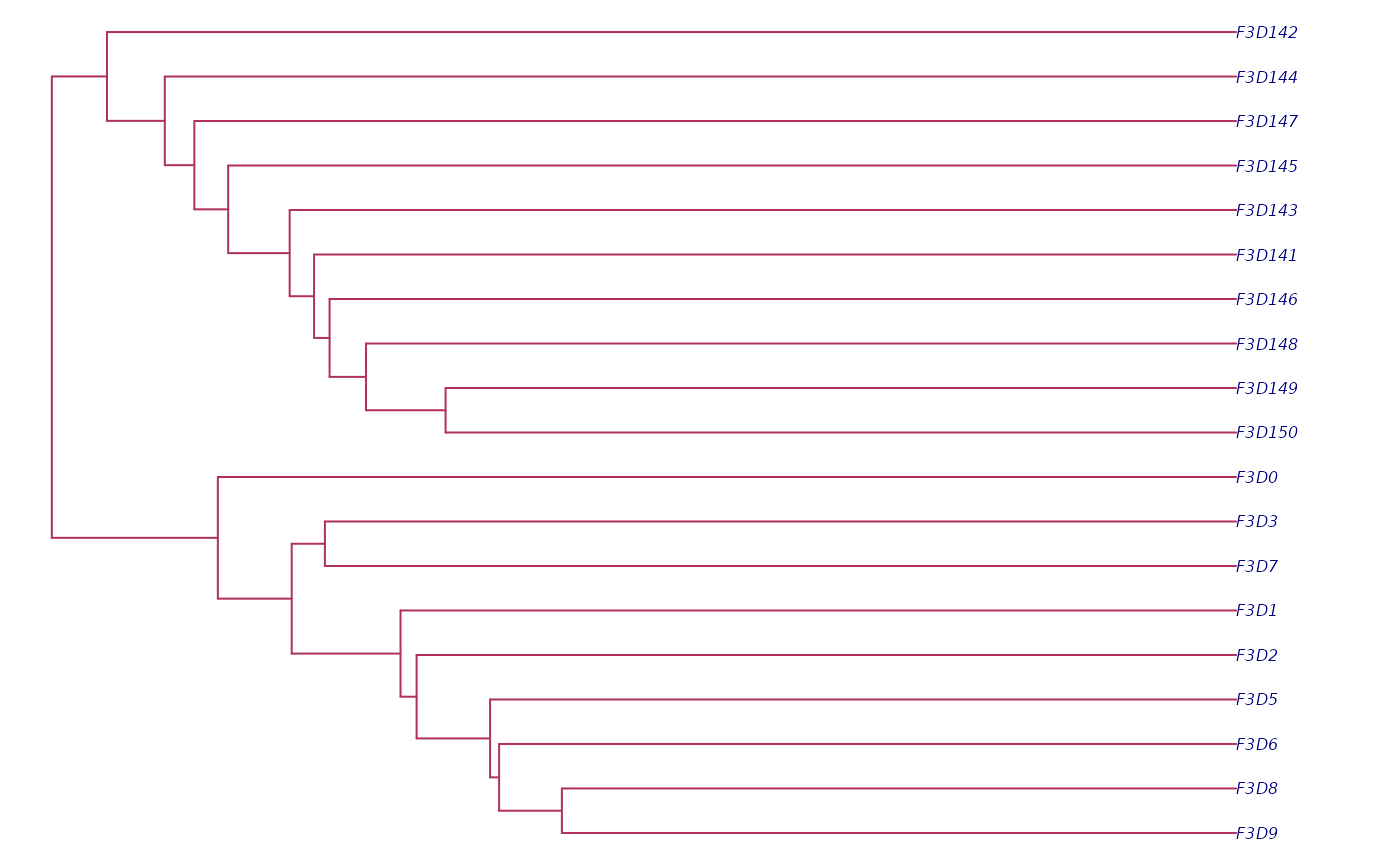
par(old_par)Thanks for following along. Next, find out how to import your own data using the links below: