The strollur package stores data associated with your Amplicon Sequence analysis. This tutorial will familiarize you some of with the functions available in the strollur package. If you haven’t reviewed the “Getting Started” tutorial, we recommend you start there.
Creating a new dataset
First let’s create an empty data set named my_data.
data <- new_dataset(dataset_name = "my_data")Importing Data
The strollur package includes two functions to allow you to add sequence data.
add() - The add function allows you to add sequences,
reports, metadata, and resource references to your data set.
assign() - The assign function allows assign sequence
abundances, sequence classifications, bins, bin representative
sequences, bin classifications, samples and treatments to your data
set.
add
The add function allows you to add sequences, reports, metadata, and resource references to your data set.
Adding FASTA sequences
First, let’s add some FASTA data.
strollur has a function for reading FASTA files named
read_fasta(). We will use it to read the sequence data into
a data.frame.
fasta_data <- strollur::read_fasta(strollur_example("final.fasta.gz"))
str(fasta_data)
#> 'data.frame':    2425 obs. of  2 variables:
#>  $ sequence_name: chr  "M00967_43_000000000-A3JHG_1_2101_16474_12783" "M00967_43_000000000-A3JHG_1_1113_12711_3318" "M00967_43_000000000-A3JHG_1_2108_14707_9807" "M00967_43_000000000-A3JHG_1_1110_4126_16552" ...
#>  $ sequence     : chr  "TAC--GG-AG-GAT--GCG-A-G-C-G-T-T--AT-C-CGTGAT--TT-A-T-T--GG-GT--TT-A-AA-GG-GT-GC-G-TA-GGC-G-G-A-CA-G-T-T-AA-G-T-"| __truncated__ "TAC--GT-AG-GGG--GCA-A-G-C-G-T-T--AT-C-CGG-AT--TT-A-C-T--GG-GT--GT-A-AA-GG-GA-GC-G-TA-GGC-G-G-C-CA-T-G-C-AA-G-T-"| __truncated__ "TAC--GG-AG-GAT--GCG-A-G-C-G-T-T--AT-C-CGG-AT--TT-A-C-T--GG-GT--GT-A-AA-GG-GA-GC-G-TA-GAC-G-G-C-GG-C-G-C-AA-G-T-"| __truncated__ "TAC--GG-AG-GAT--TCA-A-G-C-G-T-T--AT-C-CGG-AT--TT-A-T-T--GG-GT--TT-A-AA-GG-GT-GC-G-TA-GGC-G-G-G-CT-G-T-T-AA-G-T-"| __truncated__ ...

add(
  data,
  table = fasta_data,
  type = "sequence"
)
#> Added 2425 sequences.
data
#> my_data:
#>
#>             starts ends nbases ambigs polymers numns numseqs
#> Minimum:         1  375    249      0        3     0    1.00
#> 2.5%-tile:       1  375    252      0        4     0   60.62
#> 25%-tile:        1  375    252      0        4     0  606.25
#> Median:          1  375    253      0        4     0 1212.50
#> 75%-tile:        1  375    253      0        5     0 1818.75
#> 97.5%-tile:      1  375    254      0        6     0 2364.38
#> Maximum:         1  375    256      0        6     0 2425.00
#> Mean:            1  375    252      0        4     0 1212.64
#>
#> Number of unique seqs: 2425
#> Total number of seqs: 2425
If you want to include a resource reference about your fasta data you
can use the new_reference function and the reference
parameter. strollur does not allow you to add sequences with the same
name, so let’s use the clear() function to remove all data
from our data set.
clear(data)
#>
#> Total number of seqs: 0

documentation_url <- "https://mothur.org/wiki/silva_reference_files/"
method_url <- "https://mothur.org/blog/2024/SILVA-v138_2-reference-files/"

silva_resource <- new_reference(
  vendor = "SILVA",
  name = "silva.bacteria.fasta",
  version = "1.38.1",
  usage = "alignment of sequences",
  note = "reference trimmed to V4 region",
  documentation_url = documentation_url,
  method_url = method_url
)

add(
  data,
  table = fasta_data,
  type = "sequence",
  reference = silva_resource
)
#> Added 2425 sequences.
#> Added 1 resource references.
data
#>             starts ends nbases ambigs polymers numns numseqs
#> Minimum:         1  375    249      0        3     0    1.00
#> 2.5%-tile:       1  375    252      0        4     0   60.62
#> 25%-tile:        1  375    252      0        4     0  606.25
#> Median:          1  375    253      0        4     0 1212.50
#> 75%-tile:        1  375    253      0        5     0 1818.75
#> 97.5%-tile:      1  375    254      0        6     0 2364.38
#> Maximum:         1  375    256      0        6     0 2425.00
#> Mean:            1  375    252      0        4     0 1212.64
#>
#> Number of unique seqs: 2425
#> Total number of seqs: 2425
#>
#> Total number of resource references: 1
Adding Custom Reports
You may want to add custom reports to your data set such as an contigs assembly report, chimera report or alignment report. You can do so by setting type = “report”. You must also provide a report_type.
This is also a good time to explain what the table_names parameter does for you. strollur expects the columns in custom reports to have specific names. If your table’s names differ from what strollur is expecting, you will see an error like that below.
contigs_report <- readRDS(strollur_example("miseq_contigs_report.rds"))

add(
  data,
  table = contigs_report,
  type = "report",
  report_type = "contigs_report"
)

# Error: The report must include a column containing sequence names.
# sequence_names is not a named column in your report.

# Called from: xdev_add_report(data, table = table, type = report_type,
#    sequence_name = table_names[["sequence_name"]], verbose)
You can use the table_names parameter to tell strollur what the specific column is called in your custom report table. In the contigs_report the sequence_name column is called Name, so we will add one more line to the add function.
contigs_report <- readRDS(strollur_example("miseq_contigs_report.rds"))
str(contigs_report)
#> spc_tbl_ [2,425 × 8] (S3: spec_tbl_df/tbl_df/tbl/data.frame)
#>  $ Name           : chr [1:2425] "M00967_43_000000000-A3JHG_1_1101_18044_1900" "M00967_43_000000000-A3JHG_1_1101_15533_5293" "M00967_43_000000000-A3JHG_1_1101_18278_3345" "M00967_43_000000000-A3JHG_1_1101_22681_5598" ...
#>  $ Length         : num [1:2425] 253 253 253 253 253 252 253 253 253 253 ...
#>  $ Overlap_Length : num [1:2425] 249 249 249 250 249 249 249 249 249 249 ...
#>  $ Overlap_Start  : num [1:2425] 2 2 2 2 2 2 2 2 2 2 ...
#>  $ Overlap_End    : num [1:2425] 251 251 251 252 251 251 251 251 251 251 ...
#>  $ MisMatches     : num [1:2425] 5 0 1 1 0 14 0 0 3 0 ...
#>  $ Num_Ns         : num [1:2425] 0 0 0 0 0 0 0 0 0 0 ...
#>  $ Expected_Errors: num [1:2425] 0.07459 0.00215 0.00484 0.00379 0.0022 ...
#>  - attr(*, "spec")=
#>   .. cols(
#>   ..   Name = col_character(),
#>   ..   Length = col_double(),
#>   ..   Overlap_Length = col_double(),
#>   ..   Overlap_Start = col_double(),
#>   ..   Overlap_End = col_double(),
#>   ..   MisMatches = col_double(),
#>   ..   Num_Ns = col_double(),
#>   ..   Expected_Errors = col_double()
#>   .. )
#>  - attr(*, "problems")=<pointer: (nil)>

add(
  data,
  table = contigs_report,
  type = "report",
  report_type = "contigs_report",
  table_names = list(sequence_name = "Name")
)
#> Added a contigs_report report.
data
#>             starts ends nbases ambigs polymers numns numseqs
#> Minimum:         1  375    249      0        3     0    1.00
#> 2.5%-tile:       1  375    252      0        4     0   60.62
#> 25%-tile:        1  375    252      0        4     0  606.25
#> Median:          1  375    253      0        4     0 1212.50
#> 75%-tile:        1  375    253      0        5     0 1818.75
#> 97.5%-tile:      1  375    254      0        6     0 2364.38
#> Maximum:         1  375    256      0        6     0 2425.00
#> Mean:            1  375    252      0        4     0 1212.64
#>
#> Number of unique seqs: 2425
#> Total number of seqs: 2425
#>
#> Total number of resource references: 1
#> Total number of custom reports: 1
Adding Metadata
Now that we have added our custom contigs assembly report, let’s learn how to add reports not tied to sequence names. We can add metadata to our data set by setting the type = “report”, report_type = “metadata”.
metadata <- readRDS(strollur_example("miseq_metadata.rds"))
str(metadata)
#> spc_tbl_ [19 × 2] (S3: spec_tbl_df/tbl_df/tbl/data.frame)
#>  $ sample        : chr [1:19] "F3D0" "F3D1" "F3D141" "F3D142" ...
#>  $ days_post_wean: num [1:19] 0 1 141 142 143 144 145 146 147 148 ...
#>  - attr(*, "spec")=
#>   .. cols(
#>   ..   sample = col_character(),
#>   ..   days_post_wean = col_double()
#>   .. )
#>  - attr(*, "problems")=<pointer: (nil)>

add(
  data,
  table = metadata,
  type = "report",
  report_type = "metadata"
)
#> Added a metadata report.
Adding Resource References
We can add additional resource references to our data set by setting the type = “resource_reference”.
reference <- readr::read_csv(strollur_example("references.csv"),
  col_names = TRUE, show_col_types = FALSE
)

add(
  data,
  table = reference,
  type = "resource_reference"
)
#>
#> The dataset already contains a resource_reference named 'silva.bacteria.fasta', overwriting existing reference.
#>
#> Added 1 resource references.
assign
The assign() function allows assign sequence abundances,
sequence classifications, bins, bin representative sequences, bin
classifications, samples and treatments to your data set.
Assigning Abundances
After adding your FASTA sequences, you can assign abundance and sample data using the assign function with the type = “sequence_abundance”.
abundance_table <- readRDS(strollur_example("miseq_abundance_by_sample.rds"))
str(abundance_table)
#> spc_tbl_ [5,539 × 4] (S3: spec_tbl_df/tbl_df/tbl/data.frame)
#>  $ sequence_name: chr [1:5539] "M00967_43_000000000-A3JHG_1_2101_16474_12783" "M00967_43_000000000-A3JHG_1_1113_12711_3318" "M00967_43_000000000-A3JHG_1_2108_14707_9807" "M00967_43_000000000-A3JHG_1_1110_4126_16552" ...
#>  $ abundance    : num [1:5539] 1 1 1 1 1 1 22 19 12 9 ...
#>  $ sample       : chr [1:5539] "F3D150" "F3D142" "F3D3" "F3D8" ...
#>  $ treatment    : chr [1:5539] "Late" "Late" "Early" "Early" ...
#>  - attr(*, "spec")=
#>   .. cols(
#>   ..   names = col_character(),
#>   ..   abundances = col_double(),
#>   ..   samples = col_character(),
#>   ..   treatments = col_character()
#>   .. )
#>  - attr(*, "problems")=<pointer: (nil)>

assign(data, table = abundance_table, type = "sequence_abundance")
#> Assigned 2425 sequence abundances.

data
#>             starts ends nbases ambigs polymers numns   numseqs
#> Minimum:         1  375    249      0        3     0      1.00
#> 2.5%-tile:       1  375    252      0        4     0   2849.08
#> 25%-tile:        1  375    252      0        4     0  28490.75
#> Median:          1  375    253      0        4     0  56981.50
#> 75%-tile:        1  375    253      0        5     0  85472.25
#> 97.5%-tile:      1  375    254      0        6     0 111113.93
#> Maximum:         1  375    256      0        6     0 113963.00
#> Mean:            1  375    252      0        4     0  56981.64
#>
#> Number of unique seqs: 2425
#> Total number of seqs: 113963
#>
#> Total number of samples: 19
#> Total number of treatments: 2
#> Total number of resource references: 2
#> Total number of custom reports: 2
Assigning Bins
As you can see we now have abundances, samples and treatments added to the data set. Next, let’s assign the sequences to bins using type = “bin”. When you assign sequences to bins you must provide a bin_type. The bin_type is a tag of your choosing used to reference the bin clusters you are adding. Let’s add some Operational Taxonomic Unit clusters and set the bin_type = “otu”.
bin_table <- readRDS(strollur_example("miseq_list_otu.rds"))
str(bin_table)
#> spc_tbl_ [2,425 × 2] (S3: spec_tbl_df/tbl_df/tbl/data.frame)
#>  $ bin_name     : chr [1:2425] "Otu001" "Otu001" "Otu001" "Otu001" ...
#>  $ sequence_name: chr [1:2425] "M00967_43_000000000-A3JHG_1_1111_20933_6700" "M00967_43_000000000-A3JHG_1_1113_17095_9759" "M00967_43_000000000-A3JHG_1_1114_22144_24942" "M00967_43_000000000-A3JHG_1_1112_5981_8948" ...
#>  - attr(*, "spec")=
#>   .. cols(
#>   ..   otu_id = col_character(),
#>   ..   seq_id = col_character()
#>   .. )
#>  - attr(*, "problems")=<pointer: (nil)>

assign(data, table = bin_table, type = "bin", bin_type = "otu")
#> Assigned 531 otu bins.

data
#>             starts ends nbases ambigs polymers numns   numseqs
#> Minimum:         1  375    249      0        3     0      1.00
#> 2.5%-tile:       1  375    252      0        4     0   2849.08
#> 25%-tile:        1  375    252      0        4     0  28490.75
#> Median:          1  375    253      0        4     0  56981.50
#> 75%-tile:        1  375    253      0        5     0  85472.25
#> 97.5%-tile:      1  375    254      0        6     0 111113.93
#> Maximum:         1  375    256      0        6     0 113963.00
#> Mean:            1  375    252      0        4     0  56981.64
#>
#> Number of unique seqs: 2425
#> Total number of seqs: 113963
#>
#> Total number of samples: 19
#> Total number of treatments: 2
#> Total number of otus: 531
#> Total number of resource references: 2
#> Total number of custom reports: 2
You can see from the summary, we now have 531 otus in our dataset.
Note, if you are importing data from packages that preprocess the Amplicon Sequence data into features, you can assign the feature table abundances as sequence abundances and then assign the features to Amplicon Sequence Variant clusters or asv bins.
Assigning Taxonomic Classifications
Now that we have assigned our sequences to bins, let’s assign taxonomy to our sequences.
sequence_classification_data <- read_mothur_taxonomy(
  taxonomy = strollur_example("final.taxonomy.gz")
)
str(sequence_classification_data)
#> spc_tbl_ [2,425 × 2] (S3: spec_tbl_df/tbl_df/tbl/data.frame)
#>  $ sequence_name: chr [1:2425] "M00967_43_000000000-A3JHG_1_2102_17714_13657" "M00967_43_000000000-A3JHG_1_2109_7813_4701" "M00967_43_000000000-A3JHG_1_1113_19457_3875" "M00967_43_000000000-A3JHG_1_1112_18411_17052" ...
#>  $ taxonomy     : chr [1:2425] "Bacteria(100);Firmicutes(100);Clostridia(100);Clostridiales(100);Lachnospiraceae(99);Lachnospiraceae_unclassified(99);" "Bacteria(99);Firmicutes(94);Clostridia(93);Clostridiales(93);Lachnospiraceae(90);Lachnospiraceae_unclassified(90);" "Bacteria(100);Firmicutes(100);Clostridia(100);Clostridiales(100);Lachnospiraceae(100);Johnsonella(93);" "Bacteria(100);\"Bacteroidetes\"(100);\"Bacteroidia\"(98);\"Bacteroidales\"(98);\"Porphyromonadaceae\"(97);\"Por"| __truncated__ ...
#>  - attr(*, "spec")=
#>   .. cols(
#>   ..   X1 = col_character(),
#>   ..   X2 = col_character()
#>   .. )

assign(
  data,
  table = sequence_classification_data,
  type = "sequence_taxonomy"
)
#> Assigned 2425 sequence taxonomies.
Note, when you assign taxonomy to sequences that are assigned to bins, strollur will automatically assign the bin taxonomies to be the consensus taxonomy of the sequences in the bins. You can also set bin taxonomies independently by setting the type = “bin_taxonomy”.
otu_taxonomy_data <- read_mothur_cons_taxonomy(strollur_example(
  "final.cons.taxonomy"
))
str(otu_taxonomy_data)
#> spc_tbl_ [531 × 3] (S3: spec_tbl_df/tbl_df/tbl/data.frame)
#>  $ bin_name : chr [1:531] "Otu001" "Otu002" "Otu003" "Otu004" ...
#>  $ abundance: num [1:531] 12288 8892 7794 7476 7450 ...
#>  $ taxonomy : chr [1:531] "Bacteria(100);\"Bacteroidetes\"(100);\"Bacteroidia\"(100);\"Bacteroidales\"(100);\"Porphyromonadaceae\"(100);\""| __truncated__ "Bacteria(100);\"Bacteroidetes\"(100);\"Bacteroidia\"(100);\"Bacteroidales\"(100);\"Porphyromonadaceae\"(100);\""| __truncated__ "Bacteria(100);\"Bacteroidetes\"(100);\"Bacteroidia\"(100);\"Bacteroidales\"(100);\"Porphyromonadaceae\"(100);\""| __truncated__ "Bacteria(100);\"Bacteroidetes\"(100);\"Bacteroidia\"(100);\"Bacteroidales\"(100);\"Porphyromonadaceae\"(100);Barnesiella(100);" ...
#>  - attr(*, "spec")=
#>   .. cols(
#>   ..   OTU = col_character(),
#>   ..   Size = col_double(),
#>   ..   Taxonomy = col_character()
#>   .. )

assign(
  data,
  table = otu_taxonomy_data,
  type = "bin_taxonomy",
  bin_type = "otu"
)
#> Assigned 531 otu bin taxonomies.
Assigning Bin Representatives
strollur allows you to assign a bin representative sequences to the bins in your clusters. Let’s assign bin representatives to our otu bins.
bin_reps <- readRDS(strollur_example("miseq_representative_sequences.rds"))
str(bin_reps)
#> spc_tbl_ [531 × 2] (S3: spec_tbl_df/tbl_df/tbl/data.frame)
#>  $ bin_name     : chr [1:531] "Otu001" "Otu002" "Otu003" "Otu004" ...
#>  $ sequence_name: chr [1:531] "M00967_43_000000000-A3JHG_1_1108_14299_17220" "M00967_43_000000000-A3JHG_1_1106_22705_6123" "M00967_43_000000000-A3JHG_1_1101_15533_5293" "M00967_43_000000000-A3JHG_1_1105_25642_17588" ...
#>  - attr(*, "spec")=
#>   .. cols(
#>   ..   bin_names = col_character(),
#>   ..   sequence_names = col_character()
#>   .. )
#>  - attr(*, "problems")=<pointer: (nil)>

assign(
  data,
  table = bin_reps,
  type = "bin_representative"
)
#> Assigned 531 otu bin representative sequences.
Assigning Treatments
In our case the abundance_table included treatment assignments, but you can also assign samples to treatments by setting type = “treatment”.
sample_assignments <- readRDS(strollur_example("miseq_sample_design.rds"))
str(sample_assignments)
#> spc_tbl_ [19 × 2] (S3: spec_tbl_df/tbl_df/tbl/data.frame)
#>  $ sample   : chr [1:19] "F3D0" "F3D1" "F3D141" "F3D142" ...
#>  $ treatment: chr [1:19] "Early" "Early" "Late" "Late" ...
#>  - attr(*, "spec")=
#>   .. cols(
#>   ..   samples = col_character(),
#>   ..   treatments = col_character()
#>   .. )

assign(
  data,
  table = sample_assignments,
  type = "treatment"
)
#> Assigned 19 samples to treatments.
Sample Trees and Sequence Trees
Lastly, strollur allows you to add tree that relate your samples or sequences. Let’s look at some examples together.
sample_tree <- ape::read.tree(strollur_example("final.opti_mcc.jclass.ave.tre"))
sequence_tree <- ape::read.tree(strollur_example("final.phylip.tre.gz"))

data$add_sample_tree(sample_tree)
data$add_sequence_tree(sequence_tree)

#| fig.alt: >
#|   Plot of Miseq_SOP's sample relationship tree
old_par <- par(bg = "white")
ape::plot.phylo(data$get_sample_tree(),
  no.margin = TRUE,
  cex = 0.5, edge.color = "maroon", tip.color = "navy"
)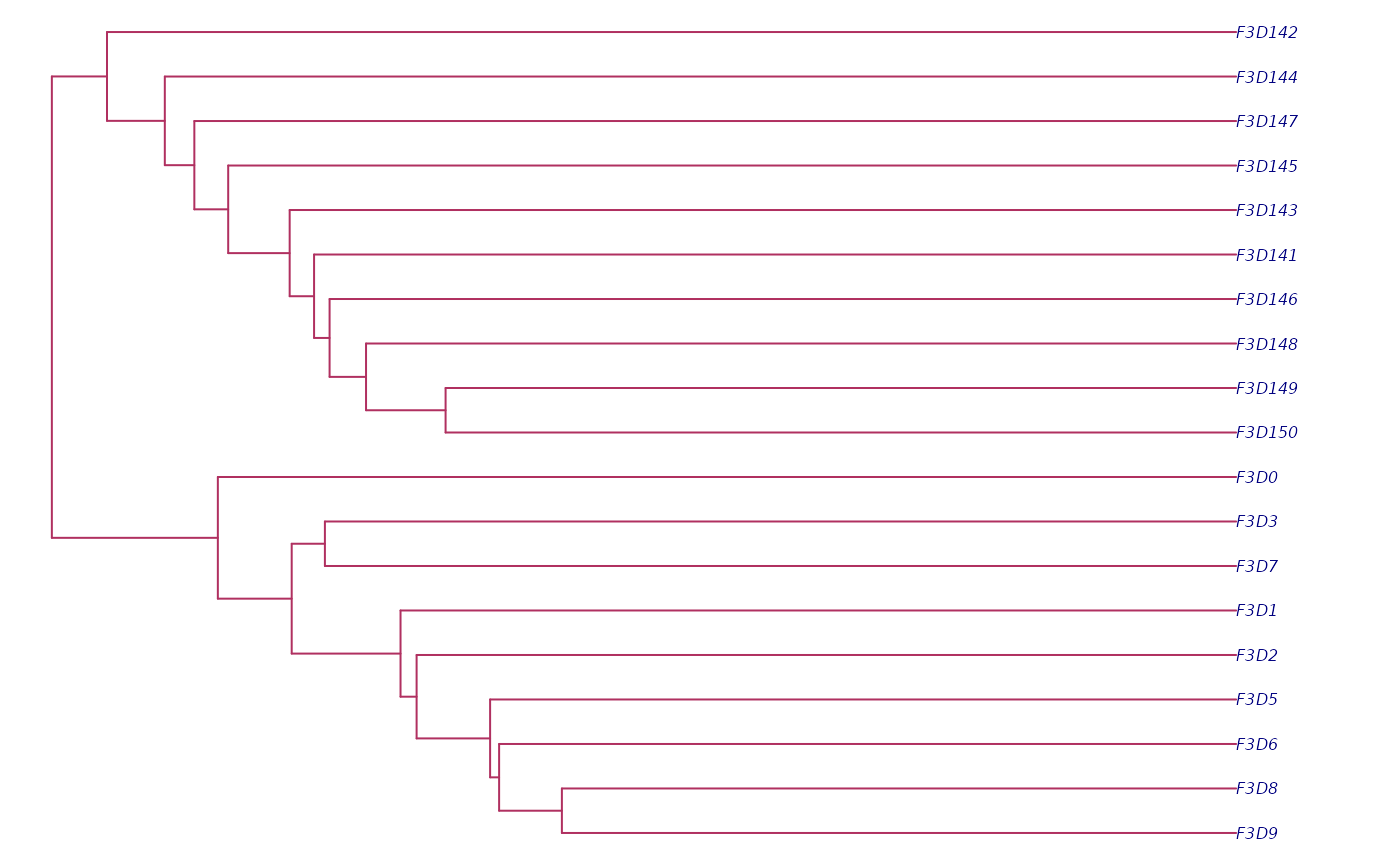
par(old_par)Thanks for following along. To learn more about the functions used to access the data in your data set, take a look at the Accessing Data tutorial.