Costello stool analysis
NOTE: This wiki page ceased to be updated after release 1.21 of mothur. Please consult the 454 SOP page for the latest and greatest method of analyzing pyrosequencing data
Recently, Costello and colleagues published a paper in Science where they sampled 9 people at four time points at 27 locations on their body. Fortunately, for us, they posted their data on the Short Read Archive. In this tutorial, I’ll use mothur to analyze the stool samples from 6 of these individuals (3 women and 3 men) showing how I would analyze the data using the methods available in mothur. Because the original sff file is not available, I’ve created mock fasta and qual files complete with the forward primer and the barcode. To follow this tutorial you will need the following files...
- costello dataset
- SILVA-based bacterial reference alignment
- SILVA-based alignment of the Gold reference set
- mothur-formatted version of the RDP training set
In addition, you probably want to get your hands on the following...
- mono - if you are using Mac OS X or linux
- catchall
- textwranger / emacs / vi / or some other text editor
- R, Excel, or another program to graph data
- Adobe Illustrator, Safari, or inkscape
- figtree or another program to visualize dendrograms
Starting out we need to first determine, what is our question? I have two. Is the variation in an individual’s microbiome greater than the variation among different individuals and do men and women harbor different microbiota. Costello and colleagues found that inter-personal variability was considerably higher than intra-personal variability; however, they did not comment on sex-based differences within a body site, except to point out that body-site differences were greater than differences due to sex. We will address these questions in this tutorial using a combination of OTU, phylotype, and phylogenetic methods. The workflow is being divided into several parts shown here in the table of contents for the tutorial:
Preprocessing
If you look within your CostelloData folder you will see four files that start with “stool”:
- stool.fasta - the V12 sequence data
- stool.qual - the quality scores for the corresponding sequences
- stool.oligos - a table that tells mothur the barcode that corresonds to each sample and the primer that was used
- stool.batch - a batch file that will be described at the end of this tutorial.
Also, it is generally easiest to use the “current” option for many of the commands since the file names get very long. Because this tutorial is meant to show people how to use mothur at a very nuts and bolts level, we will only selectively use the current option to demonstrate how it works. Generally, we will use the full file names.
Let’s go ahead and fire up mothur and get a sense of what the sequences look like using the summary.seqs command:
mothur > summary.seqs(fasta=stool.fasta, processors=2)

       Start   End NBases  Ambigs  Polymer
Minimum:   1   183 183 0   3
2.5%-tile: 1   243 243 0   4
25%-tile:  1   259 259 0   5
Median:    1   267 267 0   5
75%-tile:  1   274 274 0   5
97.5%-tile:    1   287 287 0   6
Maximum:   1   373 373 0   6
# of Seqs: 37126
There are some things to keep in mind with this analysis. Because this is a somewhat simulated dataset it has about 10-fold fewer sequences than you would normally find. Also, when you get the sequences off the sequencer, there are typically ambiguous bases and long homopolymer runs in your sequences and you will want to remove those sequence - Costello already did this for us. Note that their approach is to amplify the V1-V2 region and sequence from the 3’ end of the amplicon back towards the 27f primer. So we need to do a couple of things - i) remove the forward primer, ii) remove the barcodes, iii) remove the low quality bases, iv) create a groups file, and v) get the reverse complement of the sequences. Based on mock community experiments where known sequences are resequenced, we have found that 1 mismatch to the barcode and 2 to the primer do not adversely affect sequence quality. We have also found good correlation between the quality scores and sequencing errors between 30 and 35. There are several options for trimming sequences based on quality scores in the trim.seqs command, but the one we trust the most is to use a moving window that is 50 bp long and to require that the average quality score over the region not drop below 35. Once it does, we trim to the end of the last window with an average over 35. In mock community experiments we find that this drops the error rate by 10-fold over not trimming the sequences. In addition, we will remove any sequence where the longest homopolymer is greater than 8 nt and if it contains an ambiguous base call (i.e. an “N”).
mothur > trim.seqs(fasta=stool.fasta, oligos=stool.oligos, qfile=stool.qual, maxambig=0, maxhomop=8, flip=T, bdiffs=1, pdiffs=2, qwindowaverage=35, qwindowsize=50, processors=2)
This will generate several files - stool.trim.fasta, stool.scrap.fasta, and stool.groups. We are interested in the *trim* and *groups file for our downstream processing. Let’s see what the stool.trim.fasta and stool.scrap.fasta files look like:
mothur > summary.seqs(fasta=stool.trim.fasta)

       Start   End NBases  Ambigs  Polymer
Minimum:   1   50  50  0   2
2.5%-tile: 1   61  61  0   3
25%-tile:  1   196 196 0   5
Median:    1   220 220 0   5
75%-tile:  1   229 229 0   5
97.5%-tile:    1   240 240 0   6
Maximum:   1   243 243 0   6
# of Seqs: 35245
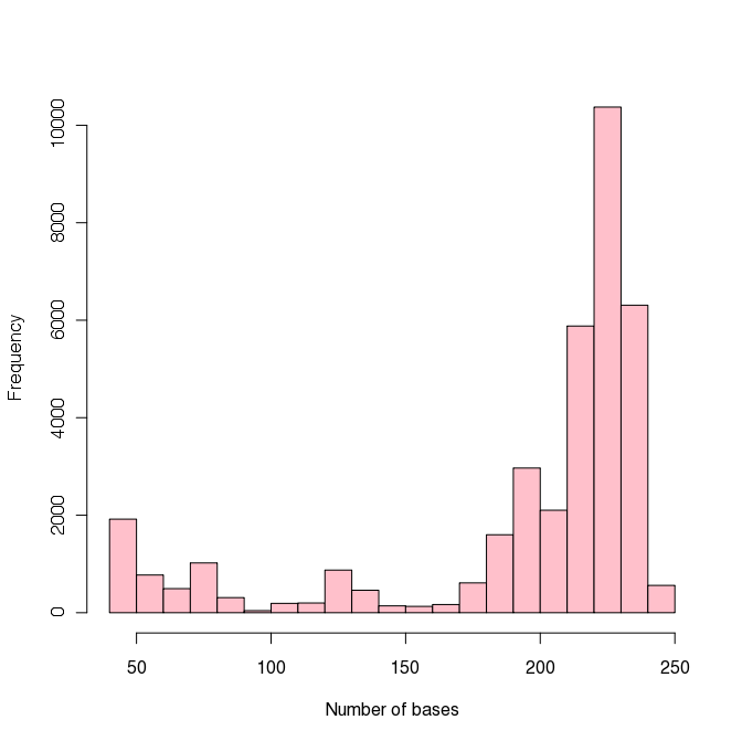
The plot to the right shows the distribution of sequence lengths. As the table above shows and the histogram emphasizes, most of the data are longer than 150 bp. We will keep this in mind for later when we want to determine the minimum sequence length that we will allow in our analysis.
Since file names can get rather long during this analysis, we have added a sort of “memory” to mothur, which will help simplify file calling. If you start with sffinfo or any other command where you insert a fasta file name, mothur will either guess which fasta file you need for the next command, or you can tell it fasta=current. The same works for name, group, accnos, and taxonomy files. In addition, if you use processors=8, mothur will remember to use 8 processors where possible in all of the other options. By using the get.current command, you can see which files mothur is identifying as the most current.
mothur > get.current()

Current files saved by mothur:
fasta=stool.trim.fasta
group=stool.groups
qfile=stool.trim.qual
Be sure to check get.current periodically to make sure mothur is using the files you intended, otherwise you may run into problems with your analysis. If you find a problem or would like to manually set your own “current” files, you can use the set.current command as follows:
mothur > set.current(fasta=stool.trim.fasta, group=stool.groups, qfile=stool.trim.qual)

 Current files saved by mothur:
 fasta=stool.trim.fasta
 group=stool.groups
 qfile=stool.trim.qual
This command can be helpful if you quit out of mothur in the middle of an analysis, or if you find that mothur isn’t using the correct files. For example, you can re-run the last summary.seqs command as follows...
mothur > summary.seqs()

Using stool.trim.fasta as input file for the fasta parameter.

       Start   End NBases  Ambigs  Polymer
Minimum:   1   50  50  0   2
2.5%-tile: 1   61  61  0   3
25%-tile:  1   196 196 0   5
Median:    1   220 220 0   5
75%-tile:  1   229 229 0   5
97.5%-tile:    1   240 240 0   6
Maximum:   1   243 243 0   6
# of Seqs: 35245

Output File Name:
stool.trim.fasta.summary
Next, we want to simplify the dataset. It is likely that a number of the 35,245 sequences are redundant. To obtain a non-redundant set of sequences, run the unique.seqs command and generate stool.trim.unique.fasta and stool.trim.names. It isn’t necessary to include the fasta file name in this command, mothur will just use the most current file:
mothur > unique.seqs(fasta=stool.trim.fasta)
You can summarize your sequences with either of the following commands:
mothur > summary.seqs(fasta=stool.trim.unique.fasta, name=stool.trim.names)

mothur > summary.seqs(fasta=current, name=current)


       Start   End NBases  Ambigs  Polymer
Minimum:   1   50  50  0   2
2.5%-tile: 1   61  61  0   3
25%-tile:  1   196 196 0   5
Median:    1   220 220 0   5
75%-tile:  1   229 229 0   5
97.5%-tile:    1   240 240 0   6
Maximum:   1   243 243 0   6
# of unique seqs:  20343
total # of seqs:   35245
We see that we have basically reduced the number of sequences that we have to align, calculate distances for, and cluster from ~35,000 to ~20,000. This will be a significant reduction that will make the analysis faster and require less memory.
Next, let’s use the SILVA-compatible alignment database and we will align the sequences using the align.seqs command and I’ll make use of the two processors on my laptop (Macs rock!). I prefer the silva reference alignment, for the reasons I articulated in a recent PLoS Computational Biology paper that I published. For now, if your computer has less than 2 GB of RAM you should probably stick with the greengenes reference alignment and tell your PI to order you some more RAM.
mothur > align.seqs(fasta=stool.trim.unique.fasta, reference=silva.bacteria.fasta, processors=2)
alternatively, you can run it as...
mothur > align.seqs(reference=silva.bacteria.fasta, processors=2)

Reading in the silva.bacteria.fasta template sequences...  DONE.
Aligning sequences...
It took 500 secs to align 20343 sequences.
The alignment is stored as a fasta-formatted file called stool.trim.unique.align and a report file that describes the alignment is given in a file called stool.trim.unique.align.report. Next, we want to see what the aligned sequences look like:
mothur > summary.seqs(fasta=current, name=current)

Using stool.trim.unique.align as input file for the fasta parameter.
Using stool.trim.names as input file for the name parameter.

       Start   End NBases  Ambigs  Polymer
Minimum:   1143    6332    50  0   2
2.5%-tile: 1776    6333    61  0   3
25%-tile:  1817    6333    196 0   5
Median:    2051    6333    220 0   5
75%-tile:  2524    6333    229 0   5
97.5%-tile:    5431    6334    240 0   6
Maximum:   5693    6334    243 0   6
# of unique seqs:  20343
total # of seqs:   35245
Based on this output, we want to maximize the number of sequences that overlap over the longest span. First, I’ll require that all of the sequences end by position 6333. We have several options for what to do next. Using the screen.seqs command we will remove any sequence that does not fit these parameters from our fasta, name, and group files. It should be mentioned that this is typically the hardest part to figure out. The tradeoff is between sequence length and the number of sequences. This is an important step because we want our sequences to fully overlap with each other.
Option 1 This is the classical appraoch. What we noticed from running summary.seqs was that pretty much every sequence ended by position 6,333. This makes sense since the researchers started downstream of the V2 region and sequenced back towards the 5’ end of the gene. We would like to set a minimum length. Based on the results of summary.seqs plotted above as a histogram, 150 bp seems reasonable as a minimum length. To do this we might run the following command:
mothur > screen.seqs(fasta=stool.trim.unique.align, name=stool.trim.names, group=stool.groups, minlength=150, end=6333)
mothur > summary.seqs(fasta=current, name=current)

Using stool.trim.unique.good.align as input file for the fasta parameter.
Using stool.trim.good.names as input file for the name parameter.

       Start   End NBases  Ambigs  Polymer
Minimum:   1143    6333    150 0   3
2.5%-tile: 1773    6333    179 0   4
25%-tile:  1817    6333    211 0   5
Median:    2042    6333    223 0   5
75%-tile:  2069    6333    229 0   5
97.5%-tile:    3108    6334    240 0   6
Maximum:   4127    6334    243 0   6
# of unique seqs:  17749
total # of seqs:   30717
You can see we removed about 13% of the sequences.
Option 2 We can remove some of the guess work by having mothur fulfil and optimise some criteria. Again, let’s set the end position at 6333 and have mothur predict the sequence length that will allow us to keep 85% of our sequences. We can do this as follows:
mothur > screen.seqs(fasta=stool.trim.unique.align, name=stool.trim.names, group=stool.groups, end=6333, optimize=minlength, criteria=85, processors=2)
mothur > summary.seqs(fasta=current, name=current)

Using stool.trim.unique.good.align as input file for the fasta parameter.
Using stool.trim.good.names as input file for the name parameter.

       Start   End NBases  Ambigs  Polymer
Minimum:   1143    6333    179 0   3
2.5%-tile: 1773    6333    184 0   4
25%-tile:  1817    6333    212 0   5
Median:    2042    6333    223 0   5
75%-tile:  2068    6333    229 0   5
97.5%-tile:    2577    6334    240 0   6
Maximum:   3161    6334    243 0   6
# of unique seqs:  17193
total # of seqs:   30025
We can see that the minimum length required to keep 85% of the sequences was 179 bp.
Option 3 One problem with optimizing the number of sequences based on the minimum length is that sequences (especially in the V1 region) vary in length when they cover the same region. So it makes more sense to optimize the number of sequences by the start position. We can do this as follows:
mothur > screen.seqs(fasta=stool.trim.unique.align, name=stool.trim.names, group=stool.groups, end=6333, optimize=start, criteria=85, processors=2)
mothur > summary.seqs(fasta=current, name=current)

Using stool.trim.unique.good.align as input file for the fasta parameter.
Using stool.trim.good.names as input file for the name parameter.

       Start   End NBases  Ambigs  Polymer
Minimum:   1143    6333    162 0   3
2.5%-tile: 1773    6333    184 0   4
25%-tile:  1817    6333    212 0   5
Median:    2042    6333    223 0   5
75%-tile:  2068    6333    229 0   5
97.5%-tile:    2577    6334    240 0   6
Maximum:   3108    6334    243 0   6
# of unique seqs:  17195
total # of seqs:   30022
By this approach all of our sequences start by position 3108 and we will be assured after we filter the ends of our sequences that our sequences are at least 162 bases in length. Although a bit of finesse and taste figures in here, Option 3 is what we’ll choose as the basis for the remainder of the analysis. Running screen.seqs created several files that will be useful in downstream analyses:
- stool.trim.unique.good.align
- stool.trim.unique.bad.accnos
- stool.trim.good.names
- stool.good.groups
We can see that we are left with ~80% of the original sequences. Keep in mind that because the sequences were filtered considerably before we started these percentages are idealized. In reality, you should expect to lose more sequences. Don’t shoot the messanger, tell Roche to stop inflating the number of sequence reads and read length.
Note that if you were using the current option, Option 3 would have been entered as:
mothur > screen.seqs(fasta=current, name=current, group=current, end=6333, optimize=start, criteria=85, processors=2)
Previously, this was the point where we would have done chimera checking. We’re going to hold off on chimera checking until later when we have finished processing the sequences. Next, we need to trim the sequences so that they overlap in the same alignment space. This is a critical step because if one compares sequences that do not overlap the same region, but rather extend into other regions, you are essentially assuming that the 16S rRNA gene sequence evolves unifromly across its length. This is definitely not true. We will do this using the filter.seqs command to remove any column that contains at least 1 “.” in it. The “.” indicates that the sequence has yet to begin or that it has already ended:
mothur > filter.seqs(fasta=stool.trim.unique.good.align, vertical=T, trump=., processors=2)

Length of filtered alignment: 374
Number of columns removed: 49626
Length of the original alignment: 50000
Number of sequences used to construct filter: 17195
This will generate the filter file (stool.filter) and the filtered fasta-formatted file (stool.trim.unique.good.filter.fasta). Now let’s see how long the sequences are:
mothur > summary.seqs(fasta=current, name=current)

       Start   End NBases  Ambigs  Polymer
Minimum:   1   374 157 0   3
2.5%-tile: 1   374 171 0   3
25%-tile:  1   374 179 0   4
Median:    1   374 179 0   5
75%-tile:  1   374 180 0   5
97.5%-tile:    1   374 184 0   6
Maximum:   1   374 196 0   6
# of unique seqs:  17195
total # of seqs:   30022
I have found that trimming sequences so that they overlap over the same region generates new duplicate sequences that weren’t detected the first go around. So let’s re-run the unique.seqs command making sure to use the name option so that our previous name file is included:
mothur > unique.seqs(fasta=stool.trim.unique.good.filter.fasta, name=stool.trim.good.names)

mothur > summary.seqs(fasta=current, name=current)

       Start   End NBases  Ambigs  Polymer
Minimum:   1   374 157 0   3
2.5%-tile: 1   374 171 0   3
25%-tile:  1   374 179 0   4
Median:    1   374 179 0   5
75%-tile:  1   374 180 0   5
97.5%-tile:    1   374 184 0   6
Maximum:   1   374 196 0   6
# of unique seqs:  8537
total # of seqs:   30022
Now we are left with two new files as output from unique.seqs:
- stool.trim.unique.good.filter.unique.fasta
- stool.trim.unique.good.filter.names
In a published paper called “Ironing out the wrinkles in the rare biosphere through improved OTU clustering” in Environmental Microbiology, Sue Huse, Mitch Sogin, and colleagues suggest using a preclustering step to reduce sequencing noise from pyrosequencing data. The basic idea is that abundant sequences are likely to generate sequences that are less abundant and differ from the dominant sequence type by about one base every 100 bases. We have implemented our version of this algorithm in the pre.cluster command. We will use it here...
mothur > pre.cluster(fasta=stool.trim.unique.good.filter.unique.fasta, name=stool.trim.unique.good.filter.names, diffs=1)

Total number of sequences before precluster was 8537.
pre.cluster removed 2899 sequences.

mothur > summary.seqs(fasta=current, name=current)

       Start   End NBases  Ambigs  Polymer
Minimum:   1   374 157 0   3
2.5%-tile: 1   374 171 0   3
25%-tile:  1   374 179 0   4
Median:    1   374 179 0   5
75%-tile:  1   374 180 0   5
97.5%-tile:    1   374 184 0   6
Maximum:   1   374 196 0   6
# of unique seqs:  5638
total # of seqs:   30022
Now that we have reduced the sequencing error rate as low as we can and we know the frequency of each sequence type, it is time to check for chimeras. Many programs (e.g. Bellerophon, UChime, Pintail, etc.) are available for identifying chimeras, but the either do not scale well or do a poor job. Here we will show you how to use both chimera.slayer and chimera.uchime to check for chimeras. If you are going to use the database-based approaches, the developers at the Broad institute and of UChime suggest using their Gold sequence database. We provide a silva-compatible alignment of this sequence collection with the silva reference files...
First, we will use chimera.slayer with a database. To do this we will first need to apply the filter we created above in filter.seqs to silva.gold.align so that the alignments are the same length:
mothur > filter.seqs(fasta=silva.gold.align, hard=stool.filter, processors=2)
then we will need to run chimera.slayer
mothur > chimera.slayer(fasta=stool.trim.unique.good.filter.unique.precluster.fasta, reference=silva.gold.filter.fasta, processors=2)
By this approach we found 639 chimeras. In general, the number of chimeras detected may vary a bit from run to run since there is a randomization procedure involved.
Alternatively, we could use chimera.slayer, but with our sequence collection as its own database. This is probably the best way of running it; however, you have to have a name file to tell the function the frequency of each sequence. One advantage of this approach is that you aren’t dependent on a database meaning that it should work for archaeal 16S and other genes as well:
mothur > chimera.slayer(fasta=stool.trim.unique.good.filter.unique.precluster.fasta, name=stool.trim.unique.good.filter.unique.precluster.names)
By this approach we found 1783 chimeras. Although this approach is better than the database approach, it is not possible to parallelize the step and it generally runs slower. For example, this command took ~2,800 seconds to run whereas the previous command took ~250 seconds.
Second, we will use Uchime with and without a database. So we can run the following...
mothur > chimera.uchime(fasta=stool.trim.unique.good.filter.unique.precluster.fasta, reference=silva.gold.ng.fasta, processors=2)
By this approach we found 1,227 chimeras.
Alternatively, we can use the sequence collection as its own database as we did with chimera.slayer:
mothur > chimera.uchime(fasta=stool.trim.unique.good.filter.unique.precluster.fasta, name=stool.trim.unique.good.filter.unique.precluster.names)
By this approach we found 1,924 chimeras in 309 seconds. Just so you know, if you use the Uclust package, the Uchime implementation there is faster. We’re using the public domain open source version of the code, which is slower (but clearly, still fast). For the purposes of this tutorial we’ll use this last approach, which generates the files stool.trim.unique.good.filter.unique.precluster.fasta.uchime.chimera and stool.trim.unique.good.filter.unique.precluster.fasta.uchime.accnos. Now we want to use the remove.seqs command to remove the chimeric sequences from our orignial fasta, names, and groups files:
mothur > remove.seqs(accnos=stool.trim.unique.good.filter.unique.precluster.fasta.uchime.accnos, fasta=stool.trim.unique.good.filter.unique.precluster.fasta, name=stool.trim.unique.good.filter.unique.precluster.names, group=stool.good.groups)

Removed 2505 sequences.
This command will generate:
- stool.trim.unique.good.filter.unique.precluster.pick.names
- stool.trim.unique.good.filter.unique.precluster.pick.fasta
- stool.good.pick.groups
As the output from remove.seqs indicates, 2505 total sequences were removed as being chimeric. Compared to the number of sequecnes in stool.good.groups (30,022), you can see that the number of sequences drops by about 8%. The Broad developers report that this is within the range of what is reasonable to expect. Although we are still processing 30,022 sequences, there are only 3,714 unique sequences.
Next we want to classify our sequences and see if there are any sequences that don’t make “sense”. For example, if we found Cyanobacteria in stool, then we’d be reasonably confident that the DNA was there as a holdover from the subject’s diet. First we are going to classify our sequences using the mothur-formatted version of the RDP training set. The default is to do 100 iterators; however, if our threshold bootstrap value is 80%, then the confidence interval will be
1.95 times the square root of (0.8 * 0.2) / 100 or 0.078. This means that the confidence interval around 80% is 72 to 88%. Alternatively, we can increase our confidence in the bootstrap value by increasing the number of iterations to 1000. Our confidence interval would shrink to 78-82%. The downside is that the operation will take ten times longer:
mothur > classify.seqs(fasta=stool.trim.unique.good.filter.unique.precluster.pick.fasta, template=trainset6_032010.rdp.fasta, taxonomy=trainset6_032010.rdp.tax, processors=2, iters=1000)
This will create:
- stool.trim.unique.good.filter.unique.precluster.pick.rdp.taxonomy
- stool.trim.unique.good.filter.unique.precluster.pick.rdp.tax.summary
Open stool.trim.unique.good.filter.unique.precluster.pick.rdp.tax.summary and scroll to the bottom. You’ll find two unique sequences that affiliate with Chloroplasts (despite people that insist on saying “microflora”, there’s no functional flora in the gut and Chloroplasts are not bacteria). We’d like to remove these from our analysis:
mothur > remove.lineage(fasta=stool.trim.unique.good.filter.unique.precluster.pick.fasta, name=stool.trim.unique.good.filter.unique.precluster.pick.names, group=stool.good.pick.groups, taxonomy=stool.trim.unique.good.filter.unique.precluster.pick.rdp.taxonomy, taxon=Cyanobacteria)
Because there were several copies of the unique cyanobacterial sequences, we ended up removing 5 sequences from subsequent analysis. At this point we have four files that we will need for all of our downstream processing:
- stool.trim.unique.good.filter.unique.precluster.pick.rdp.pick.taxonomy
- stool.trim.unique.good.filter.unique.precluster.pick.pick.names
- stool.trim.unique.good.filter.unique.precluster.pick.pick.fasta
- stool.good.pick.pick.groups
These are some pretty gangly file names. Let’s rename these files to something simpler using mothur’s system command (if you’re using windows use copy instead of cp):
mothur > system(cp stool.trim.unique.good.filter.unique.precluster.pick.rdp.pick.taxonomy stool.final.taxonomy)
mothur > system(cp stool.trim.unique.good.filter.unique.precluster.pick.pick.names stool.final.names)
mothur > system(cp stool.trim.unique.good.filter.unique.precluster.pick.pick.fasta stool.final.fasta)
mothur > system(cp stool.good.pick.pick.groups stool.final.groups)
Now we’re done with the pre-processing steps. At this point we know that we have a collection of high quality sequences spanning the V2 region and part of the V1 region. If you have followed all of the steps I have outlined here, you will have reduced your error rate from ~0.80% to ~0.02%.
Sequence analysis
There are three general approaches for analyzing the sequences that we have been curating:
- OTU-based analsysis
- Phylotype-based analysis
- Phylogeny-based aanlysis
OTU-based analysis
Now we want to use our high quality sequences to generate a distance matrix. To do this we will use the dist.seqs command:
mothur > dist.seqs(fasta=stool.final.fasta, cutoff=0.25, processors=2)
Now we are ready to assign our sequences to OTUs using the cluster command with the average neighbor algorithm:
mothur > cluster(column=stool.final.dist, name=stool.final.names)
This command will take about a minute to run and will provide some output as it goes along. This output is also found in the stool.final.an.sabund file. In addition a stool.final.an. rabund and stool.final.an.list file are generated as well. If the distance matrix is larger than the amount of RAM your computer has, you can also use the hcluster command. This has a small memory footprint, but can take considerably longer to run than the cluster command.
mothur > hcluster(column=current, name=current, cutoff=0.25, method=average)
The output should be more or less the same as you get with the cluster command.
Alternatively, you can use the cluster.split command, which is a heuristic, but very accurate and fast...
mothur > cluster.split(taxonomy=stool.final.taxonomy, name=stool.final.names, fasta=stool.final.fasta, taxlevel=3, processors=2)
Now that we have assigned all of the sequences to OTUs we are interested in calculating the coverage, richness, and diversity of each sample. The first step is to use our group file (stool.final.groups) to parse the list file (stool.final.an.list). I like to do my analysis at a cutoff level of 0.10, but you are free to use whatever you want. To do the parsing, we will use the make.shared command with the list and group options:
mothur > make.shared(list=stool.final.an.list, group=stool.final.groups, label=0.03)
This will generate 24 rabund files (one for each of the samples) and a shared file. Opening stool.final.an.shared you’ll find that there are about 1,330 OTUs that were found across all of the samples. We would like to know “who” these OTUs are. Our preferred approach to this is the classify.otu command:
mothur > classify.otu(taxonomy=stool.final.taxonomy, name=stool.final.names, list=stool.final.an.list, label=0.03)
This will generate stool.final.an.0.03.cons.taxonomy. The first six lines of this file will look something like the following:
OTU    Size    Taxonomy
1  2088    Bacteria(100);"Bacteroidetes"(100);"Bacteroidia"(100);"Bacteroidales"(100);Bacteroidaceae(100);Bacteroides(100);
2  2178    Bacteria(100);"Bacteroidetes"(100);"Bacteroidia"(100);"Bacteroidales"(100);Bacteroidaceae(100);Bacteroides(100);
3  1209    Bacteria(100);"Bacteroidetes"(100);"Bacteroidia"(100);"Bacteroidales"(100);Bacteroidaceae(100);Bacteroides(100);
4  615 Bacteria(100);"Bacteroidetes"(100);"Bacteroidia"(100);"Bacteroidales"(100);Bacteroidaceae(100);Bacteroides(100);
5  1464    Bacteria(100);"Bacteroidetes"(100);"Bacteroidia"(100);"Bacteroidales"(100);Bacteroidaceae(100);Bacteroides(100);
This tells us that the first OTU contained 2,088 sequences and all of them were classified as Bacteroides. Notice that four of these five OTUs have the same genus level classification indicating that these OTUs represent sub-OTU lineages.
Phylotype-based analyses
Earlier we ran classify.seqs. After removing the cyanobacterial sequences were left with the contents of stool.final.taxonomy. Openning this file we see the following on the first five lines:
M14Fcsw_240901 Bacteria(100);"Bacteroidetes"(100);"Bacteroidia"(100);"Bacteroidales"(100);Bacteroidaceae(100);Bacteroides(100);
F14Fcsw_190287 Bacteria(100);"Bacteroidetes"(99.9);"Bacteroidia"(99.8);"Bacteroidales"(99.8);Bacteroidaceae(97.5);Bacteroides(97.5);
M23Fcsw_69899  Bacteria(100);"Bacteroidetes"(100);"Bacteroidia"(100);"Bacteroidales"(100);Bacteroidaceae(100);Bacteroides(100);
F31Fcsw_330793 Bacteria(100);"Bacteroidetes"(100);"Bacteroidia"(100);"Bacteroidales"(100);Bacteroidaceae(99.9);Bacteroides(99.9);
F31Fcsw_318100 Bacteria(100);"Bacteroidetes"(99.9);"Bacteroidia"(99.9);"Bacteroidales"(99.9);Bacteroidaceae(99.3);Bacteroides(99.3);
These data show us the taxonomy information for five sequences along with the number of bootstrap replicates that gave the same taxonomy output. Clearly these are all high confidence taxonomic assignments. The benefit of having used the RDP training set is that the taxonomy is base upon the Linnean model providing classification from the levels of Kingdom to Genus. If the bootstrap value drops below 80% for a level, then the next highest level with a bootstrap value above 80% is returned. Go ahead and open the file stool.final.rdp6.tax.summary. You’ll notice that this file is a gigantic table containing the various taxonomic lineages found in the dataset as well as the number of sequences that correspond to each lineage.
To carry out the phylotype analysis, we would like to convert this table into a list file so that we can perform an analysis in parallel with the OTU-based analysis. We can do this with the phylotype command:
mothur > phylotype(taxonomy=stool.final.taxonomy, name=stool.final.names)
Instead of listing the membership of each OTU using distance-based cutoffs in the file stool.final.tx.list, the phylotype command generates the data at different levels within the hierarchy. Using the rdp6 taxonomy outline you will find 6 taxonomic levels - level 1 corresponds to the level of genus and 6 is the domain (i.e. Bacteria). To generate the shared file, we again use make.shared:
mothur > make.shared(list=stool.final.tx.list, group=current, label=1)
Looking at the stool.final.tx.shared file we can see that there were only 198 phylotypes. Again, we can run classify.otu to determine the identity of each phylotype:
mothur > classify.otu(taxonomy=stool.final.taxonomy, name=current, list=stool.final.tx.list, label=1)
Phylogenetic-based analyses
The phylogenetic-based methods are based on a phylogenetic tree to calculate measures of alpha and beta-diversity. These are the metrics that Costello and her colleagues employed in most of their analyses. In the original Costello manuscript and pretty much every other paper that uses these metrics a Lane mask is applied. Here, we’ll repeat that analysis without using a Lane mask; although the Lane mask is useful for discriminating at broad phylogenetic levels, here we are interested in performing a fine-level analysis. As we have shown previously, using a Lane mask can significantly reduce the overall genetic diversity in the dataset and have the effect of making things look more similar than they are. First, we will need to create a phylip-formatted distance matrix from our sequences:
mothur > dist.seqs(fasta=stool.final.fasta, output=lt, processors=2)
Next, we will use clearcut within the mothur environment:
mothur > clearcut(phylip=stool.final.phylip.dist)
This command will produce a file called stool.final.phylip.tre.
Sample analysis
Having used our sequenes to generate OTUs, phylotypes, and a phylogenetic tree we now need to analyze these data to address our original questions. There are several approaches we can take to analyzing our samples based on these approaches. First, we can use metrics of traditional alpha and beta diversity and population-level differences. Second, we can use a variety of data visualization tools to help interpret the results. Third, there are a number of tools we can use to detect and explain differences observed among samples of different treatments. In this section we will describe how to use those tools using the data produced in the previous section. This is the fun part :).
OTU-based analysis
The advantage of OTU-based analyses is that they are not depenent on a pre-defined taxonomy. Furthermore, because the phylotype-based approach can only assign sequences to the level of Genus, it is likely that with a well-chosen cutoff (e.g. 0.03) we can look at sub-Genus deliniations of the community. We saw this earlier when observing that multiple OTUs classified to the same Genus.
Alpha diversity
Let’s start our analysis by analyzing the alpha diversity of the 24 samples. First we will generate collector’s curve of the Chao1 richness estimators and the inverse Simpson diversity index. To do this we will use the collect.single command. Also, because there are 704 sequences in this sample, let’s only spit data out every 5 sequences:
mothur > collect.single(shared=stool.final.an.shared, calc=chao-invsimpson, freq=5)
This command will generate 24 files ending in *.chao and *.invsimpson, which can be plotted in your favorite graphing software package. When you look at these plots you will see that the Chao1 curves continue to climb with sampling; however, the inverse Simpson diversity indices are relatively stable. In otherwords, it isn’t really possible to compare the richness of these communities based on the Chao1 index, but it is with the inverse Simpson index. As a quick aside, it is important to point out that Chao1 is really a measure of the minimum richneess in a community, not the full richness of the community. One method often used to get around this problem is to look at rarefaction curves describing the number of OTUs observed as a function of sampling effort. We’ll do this with the rarefaction.single command:
mothur > rarefaction.single(freq=5)
This will generate 24 files ending in *.rarefaction, which again can be plotted in your favorite graphing software package. Alas, rarefaction is not a measure of richness, but a measure of diversity. If you consider two communities with the same richness, but different evenness then after sampling a large number of individuals their rarefaction curves will asymptote to the same value. Since they have different evennesses the shapes of the curves will differ. Therefore, selecting a number of individuals to cutoff the rarefaction curve isn’t allowing a researcher to compare samples based on richness, but their diversity. Another alternative method where the richness estimate is not sensitive to sampling effort is to use parametric estimators of richness using the Catchall command. By increasing sampling effort, the confidence interval about the richness estimate will shrink.
mothur > catchall()
Finally, let’s get a table containing the number of sequences, the sample coverage, the number of observed OTUs, and the invsimpson diversity estimate using the summary.single command:
mothur > summary.single(calc=nseqs-coverage-sobs-invsimpson)
These data will be outputted to a table in a file called stool.final.an.groups.summary. Interestingly, the sample coverage varied between 85 and 96%, further demonstrating that the communities were not fully sampled. Inspection of the table also suggests that these 6 individuals varied considerably in their gut diversity and that the diversity of an individual’s gut diversity was more similar when sampled on adjacent days than when sampled a month apart.
Beta diversity measurements
Now we’d like to compare the membership and structure of the 24 stool communities using an OTU-based approach. Let’s start by generating a heatmap of the relative abundance of each OTU across the 24 samples using the heatmap.bin command and log2 scaling the relative abundance values. Because there are so many OTUs, let’s just look at the top 50 OTUs:
mothur > heatmap.bin(scale=log2, numotu=50)
This will generate an SVG-formatted file that can be visualized in Safari or manipulated in graphics software such as Adobe Illustrator. Needless to say these heatmaps can be a bit of Rorshock. A legend can be found at the bottom left corner of the heat map.
Now let’s calculate the similarity of the membership and structure found in the 24 communities and visualize those similarities in a heatmap with the jaccard and thetayc coefficients. We will do this with the heatmap.sim command:
mothur > heatmap.sim(calc=jclass-thetayc)
The output will be in two SVG-formatted files called stool.final.an.0.03jclass.heatmap.sim.svg and stool.final.an.0.10thetayc.heatmap.sim.svg. In all of these heatmaps the red colors indicate communities that are more similar than those with black colors.
When generating Venn diagrams we are limited by the number of samples that we can analyze simultaneously. Let’s take a look at the Venn diagrams for the first female subject using the venn command:
mothur > venn(groups=F11Fcsw-F12Fcsw-F13Fcsw-F14Fcsw)
This generates an interesting looking 4-way Venn diagram in the stool.final.fn.0.03.venn.sharedsobs.svg file. This shows that there were a total of 489 OTUs observed between the 4 time points. Only 46 of those OTUs were shared by all four time points. Let’s use two non-parametric estimators to see what the predicted minimum number of overlapping OTUs is for subject 1 using the summary.shared command:
mothur > summary.shared(calc=sharedchao, groups=F11Fcsw-F12Fcsw-F13Fcsw-F14Fcsw, all=T)
Opening the stool.final.an.sharedmultiple.summary file we see a prediction that female subject 1’s core microbiome contained at least 69 OTUs.
Next, let’s generate a dendrogram to describe the similarity of the samples to each other. We will generate a dendrogram using the jclass and thetayc calculators within the tree.shared command:
mothur > tree.shared(calc=thetayc-jclass)
This command generates two newick-formatted tree files - stool.final.an.thetayc.0.03.tre and stool.final.an.jclass.0.03.tre - that can be visualized in software like TreeView or FigTree. Inspection of the both trees shows that individuals’ communities cluster with themselves to the exclusion of the others. We can test to deterine whether the clustering within the tree is statistically significant or not using by choosing from the parsimony, unifrac.unweighted, or unifrac.weighted commands. To run these we will first need to create a design file that indicates which treatment each sample belongs to. Enter the following into a text editor window and save it to the CostelloData folder as stool.design:
F11Fcsw    F
F12Fcsw    F
F13Fcsw    F
F14Fcsw    F
F21Fcsw    F
F22Fcsw    F
F23Fcsw    F
F24Fcsw    F
F31Fcsw    F
F32Fcsw    F
F33Fcsw    F
F34Fcsw    F
M11Fcsw    M
M12Fcsw    M
M13Fcsw    M
M14Fcsw    M
M21Fcsw    M
M22Fcsw    M
M23Fcsw    M
M24Fcsw    M
M41Fcsw    M
M42Fcsw    M
M43Fcsw    M
M44Fcsw    M
Using the parsimony command:
mothur > read.tree(tree=stool.final.an.thetayc.0.03.tre, group=stool.design)
mothur > parsimony()

Tree#  Groups  ParsScore   ParsSig
1  F-M 2   <0.001

mothur > unifrac.weighted(random=T)

Tree#  Groups  WScore  WSig
1  F-M 0.934991    <0.001

mothur > unifrac.unweighted(random=T)

Tree#  Groups  UWScore UWSig
1  F-M 0.978037    <0.001
These three methods all show that there is structure within the tree that separates Men and Women.
Another popular way of visualizing beta-diversity information is through ordination plots. We can calculate distances between samples using the dist.shared command:
mothur > dist.shared(shared=stool.final.an.shared, calc=thetayc-jclass)
The two resulting distance matrices (i.e. stool.final.an.thetayc.0.03.lt.dist and stool.final.an.jclass.0.03.lt.dist) can then be visualized using the pcoa or nmds plots. Principal Coordinates (PCoA) uses an eigenvector-based approach to represent multidimensional data in as few dimesnsions as possible. Our data is highly dimensional (~22 dimensions).
mothur > pcoa(phylip=stool.final.an.thetayc.0.03.lt.dist)
mothur > pcoa(phylip=stool.final.an.jclass.0.03.lt.dist)
The output of these commands are three files ending in *dist, *pcoa, and *pcoa.loadings. The stool.final.an.thetayc.0.03.lt.pcoa.loadings file will tell you what fraction of the total variance in the data are represented by each of the axes. In this case the first and second axis represent 31 and 23% of the variation (54% total) for the thetaYC distances. The output to the screen indicates that the R-squared between the original distance matrix and the distance between the points in 2D PCoA space was 0.7000.
Alternatively, non-metric multidimensional scaling (NMDS) tries to preserve the distance between samples using a user defined number of dimensions. We can run our data through NMDS with 2 dimensions with the following commands
mothur > nmds(phylip=stool.final.an.thetayc.0.03.lt.dist)

mothur > nmds(phylip=stool.final.an.jclass.0.03.lt.dist)
Opening the stool.final.an.thetayc.0.03.lt.nmds.stress file we can inspect the stress and R2 values, which describe the quality of the ordination. Each line in this file represents a different iteration and the configuration obtained in the iteration with the lowest stress is reported in the stool.final.an.thetayc.0.03.lt.nmds.axes file. In this file we find that the lowest stress value was 0.224034 with an R-squared value of 0.7557. Going to 3 dimensions, the stress value drops in half and the R-squared value exceeds 0.90. Thus, we can conclude that, NMDS is better than PCoA. We can plot the two dimensions of the NMDS data by plotting the contents of stool.final.an.thetayc.0.03.lt.nmds.axes. Again, it is clear that individuals cluster separately from each other.
Ultimately, ordination is a data visualization tool. We might ask if the spatial separation that we see between the Men’s and Women’s plots in the NMDS plot is statistically significant. To do this we have two statistical tools at our disposal. The first analysis of molecular variance (amova), tests whether the centers of the clouds representing a group are more separated than the variation among samples of the same treatment. This is done using the distance matrices we created earlier and does not actually use ordination.
mothur > amova(phylip=stool.final.an.thetayc.0.03.lt.dist, design=stool.design)

 F-M   Among   Within  Total
SS 2.10271 5.51471 7.61742
df 1   22  23
MS 2.10271 0.250669

Fs:    8.3884
p-value: <0.001*

mothur > amova(phylip=stool.final.an.jclass.0.03.lt.dist, design=stool.design)

F-M    Among   Within  Total
SS 0.890504    7.39889 8.28939
df 1   22  23
MS 0.890504    0.336313

Fs:    2.64784
p-value: <0.001*
We can see that the observed separation in Male and Female samples is statistically significant. Another test we can perform is to determine whether the variation in the samples from Men and Women is different. This can be done using a distance-based version of Bartlett’s test for homogeneity of variance (homova):
mothur > homova(phylip=stool.final.an.thetayc.0.03.lt.dist, design=stool.design)

HOMOVA BValue  P-value SSwithin/(Ni-1)_values
F-M    0.472545    <0.001* 0.3032  0.198137

mothur > homova(phylip=stool.final.an.jclass.0.03.lt.dist, design=stool.design)

HOMOVA BValue  P-value SSwithin/(Ni-1)_values
F-M    0.00416016  0.228   0.343   0.329626
Again, we see that for the thetaYC distances, there is considerable difference in the variation of Men’s and Women’s samples. When we look at the membership of these communities we can see that the difference in intra-sex sample variation is not significant.
Next, we might ask which OTUs are responsible for shifting the samples along the two axes. We can determine this by measuring the correlation of the relative abundance of each OTU with the two axes in the NMDS dataset. We do this with the corr.axes command:
mothur > corr.axes(axes=stool.final.an.thetayc.0.03.lt.nmds.axes, shared=stool.final.an.shared, method=spearman, numaxes=2)
This command generates the stool.final.an.spearman.corr.axes file. Sort this file by the final column - “length”. The first five lines look like this...
OTU    axis1   axis2   length
1  -0.375176   -0.915127   0.989047
159    -0.030329   0.870074    0.870602
5  -0.661560   0.513914    0.837717
8  0.468745    0.671183    0.818663
38 -0.592141   0.550178    0.808286
What these results show is that OTU1 is responsible for moving points in the negative direction along axis 2 whereas OTU159 moves it along the positive direction on axis 2. Recalling that we classified each OTU earlier, we can open stool.final.an.0.03.cons.taxonomy to see that OTU1 was an OTU corresponding to members of the Bacteroides and that OTU159 was an OTU corresponding to members of the Oscillibacter. These data can be plotted in what’s known as a biplot where lines radiating from the origin (axis1=0, axis2=0) to the correlation values with each axis are mapped on top of the PCoA or NMDS plots. Later, using the metastats command, we will see another method for describing which populations are responsible for differences seen between specific treatments.
An alternative approach to building a biplot would be to provide data indicating metadata about each sample. For example, we may know the weight, height, blood pressure, etc. of the subjects in these 24 samples. These data are made up, but go ahead and copy and paste them into a file we’ll call stool.metadata:
group  weight
F11Fcsw    120
F12Fcsw    120
F13Fcsw    123
F14Fcsw    123
F21Fcsw    129
F22Fcsw    120
F23Fcsw    131
F24Fcsw    130
F31Fcsw    146
F32Fcsw    146
F33Fcsw    145
F34Fcsw    145
M11Fcsw    180
M12Fcsw    180
M13Fcsw    180
M14Fcsw    180
M21Fcsw    202
M22Fcsw    202
M23Fcsw    201
M24Fcsw    201
M41Fcsw    195
M42Fcsw    194
M43Fcsw    195
M44Fcsw    195

mothur > corr.axes(axes=stool.final.an.thetayc.0.03.lt.nmds.axes, metadata=stool.metadata, method=spearman, numaxes=2)
Opening the output file we see that these fictitious weights have close to no correlation with axis 1 and a correlation coefficient of -0.80 with axis 2. Plotting this on top of the NMDS data, we see that this is a driving force separating the samples from men and women.
population-level analysis
In addition to the use of corr.axes we can also use metastats to determine whether there are any OTUs that are differentially represented between the samples from men and women in this study. Run the following in mothur:
mothur > metastats(shared=stool.final.an.shared, design=stool.design)
Looking at the screen output for the first ten OTUs we see the following:
Feature 1 is significant, p = 0.0009990010
Feature 3 is significant, p = 0.0009990010
Feature 4 is significant, p = 0.0029970030
Feature 5 is significant, p = 0.0000000000
Feature 8 is significant, p = 0.0019980020
Feature 10 is significant, p = 0.0000000000
Looking in the stool.final.an.0.03.M-F.metastats file for these OTUs we see the following...
OTU    mean(group1)    variance(group1)    stderr(group1)  mean_of_counts(group1)  mean(group2)    variance(group2)    stderr(group2)  mean_of_counts(group1)  p-value
1  89.5    3456.2  17.7    173.8   6.9 118.1   3.0 11.6    0.0
3  29.3    524.1   6.9 52.0    0.6 3.2 0.4 1.0 0.0
4  0.0 0.0 0.0 0.0 49.3    4484.8  18.5    109.6   0.0
5  0.0 0.0 0.0 0.0 68.1    8875.9  26.1    126.3   0.0
8  0.0 0.0 0.0 0.0 14.8    440.1   5.8 32.7    0.0
10 0.0 0.0 0.0 0.0 8.5 90.3    2.6 17.6    0.0
These data tell us that OTUs 1 and 3 were over represented in men (group1) and OTUs 4, 5, 8, and 10 were over represented in women (group2). OTUs 1, 3, 4, 8, and 10 affiliate with members of the Bacteroides sp. and OTU 5 affiliates with members of the Prevotella sp. It is interesting to note that different OTUs from the same genus are differentially represented in men and women. In a phylotype-based analysis, this type of differentiation would not have been possible.
Phylotype-based analysis
Phylotype-based analysis is the same as OTU-based analysis, but at a different taxonomic scale. We will leave you on your own to replicate the OTU-based analyses described above with the contents of the stool.final.tx.shared file.
Phylogeny-based analysis
OTU and phylotype-based analyses are taxonomic approaches that depend on a binning procedure. In contrast, phylogeny-based approaches attempt similar types of analyses using a phylogenetic tree as input instead of a shared file. Because of this difference these methods compare the genetic diversity of different communities.
Alpha diversity
When using phylogenetic methods, alpha diversity is calculated as the total of the unique branch length in the tree. This is done using the phylo.diversity command:
mothur > phylo.diversity(tree=stool.final.phylip.tre, name=current, group=current)
This will generate a file called stool.final.1.phylodiv.summary. Reading the last column in the file you can ascertain the amount of branch length that is contributed by each group. To replicate the figures provided by Costello you will need to rarefy the data, again using the phylo.diversity command:
mothur > phylo.diversity(rarefy=T)
Beta diversity
The unifrac-based metrics are used to assess the similarity between two communities membership (unifrac.unweighted) and structure (unifrac.weighted). We will use these metrics and generate PCoA plots to compare our 24 stool samples. There are two beta-diversity metrics that one can use - unweighted and weighted.
mothur > unifrac.unweighted(distance=lt, processors=2, random=F)
mothur > unifrac.weighted(distance=lt, processors=2, random=F)
These commands will distance matrices (stool.final.tre1.unweighted.phylip.dist and stool.final.tre1.weighted.phylip.dist) that can be analyzed using all of the ordination approaches described above.
Conclusion
There are many other ways that one could analyze the data generated by Costello and her colleagues. I encourage you to go back and change the settings, use different calculators, come up with a hypothesis using the data and test it. If you think of an analysis that you wish mothur would do, please let us know and we’ll see about adding it to the package. There is a certain “pipeline” aspect to this analysis; however, it is also very much an art of working with sequences. If you want to basically do everything that was described above, you can use the stool.batch file and use mothur in the batch mode as follows:
$ ./mothur stool.batch