Sogin data analysis
In 2006, Mitch Sogin and his colleagues at the Marine Biology Laboratory in Woods Hole, MA published a ground breaking paper in pnas, which was titled, “Microbial diversity in the deep sea and the underexplored ‘rare biosphere’. Their publication was the first to use pyrosequencing technology to sequence 16S rRNA gene tags. Specifically, they sequenced 118,000 V6 tags from the 16S rRNA gene. This region was approximately 60 bp long and was ideal for use with the GS20 454 technology available at the time. They used muscle to align the sequences, an in-house distance calculator called quickdist, and DOTUR. Because of the software restrictions it was difficult to analyze individual samples, much less make comparisons across samples. Here we describe how we would use mothur to analyze the dataset. Also, this analysis was done on my MacBook Pro laptop with 2 GB of RAM, using only one of the 2 GHz processors. Feel free to start from scratch as described below or to download all of the files that will be generated in this exercise.
Data availability
The V6 sequence tags are available from the author’s MBL website as a zip file. You can see the metadata in Table 1 of their paper. The decompressed folder will be called supplemental - rename it to something more meaningful like “sogin”. Opening the sogin folder you will see two folders - original-data and updated-20080221. The updated folder contains the result of a reanalysis of the raw sequences resulting in a total of more than 222,000 V6 tags. These are the sequences we will use in this analysis. Using the terminal, use unix commands to navigate to the updated-20080221 folder. Within this folder are 8 fasta-formatted sequence files and a readme.txt file. At the prompt type the following:
$ grep -c ">" *.fa
This will produce the following output, which indicates the number of sequences in each file:
112R.fa:16087
115R.fa:16651
137.fa:14147
138.fa:13241
53R.fa:13040
55R.fa:10134
FS312.fa:55592
FS396.fa:83399
First, we want to generate a groups file. To do this type the following commands:
$ grep ">" 112R.fa > 112R.group
$ grep ">" 115R.fa > 115R.group
$ grep ">" 137.fa > 137.group
$ grep ">" 138.fa > 138.group
$ grep ">" 53R.fa > 53R.group
$ grep ">" 55R.fa > 55R.group
$ grep ">" FS312.fa > FS312.group
$ grep ">" FS396.fa > FS396.group
Now, assuming you have a text editor like textwrangler or bbedit, type the following:
$ edit *group # for TextWrangler
or
$ bbedit *group # for BBedit
Within the text editor for each file go Search->Find... and in the “Find” window enter a ‘>’ character and leave the “Replace” window blank. Hit the “Replace all” button. Next, make sure the “Grep” box is checked. Then in the “Find” window enter ‘\r’ and in the “Replace” window type ‘\t’ followed by the name of the group (e.g. 112R) followed by a ‘\r’ [’\t112r\r]. Then hit the “Replace All” button. Close the Find window, save the file, and close it. Repeat for the remaining 7 files. Once all 8 files have been processed this way, enter the following commands in the terminal:
$ cat *.group > sogin.groups
$ cat *.fa > sogin.fasta
You now have a massive fasta-formatted file and a group file, which each have 222,291 sequences in them. You are now ready to use mothur.
Generating an alignment & distance matrix
The first thing we want to do is to deconvolute the sequences in mothur so that we aren’t analyzing all 222,291 sequences. Open mothur and enter the following command:
mothur > unique.seqs(fasta=sogin.fasta)
This will generate two files - sogin.unique.fasta and sogin.names. Each of these files has 21,908 sequences. Now we will align the sequences using mothur’s align.seqs command. Unpublished results from our lab has shown that when analyzing V6 tags, the best kmer size is 9 and the optimal alignment method is needleman with a gap-opening penalty of -1. We will use the greengenes alignment to align the sequences:
mothur > align.seqs(candidate=sogin.unique.fasta, template=core_set_aligned.imputed.fasta, ksize=9, align=needleman, gapopen=-1)
This should only take about 170 seconds to run. At the end you will have two new files - sogin.unique.kmer.needleman.nast.report and sogin.unique.kmer.needleman.nast.align. The *.report file will give you some statistics on your alignments and the *align file will give you an alignment that is compatible with the greengenes arb database. Go ahead and change the name of sogin.unique.kmer.needleman.nast.align to something shorter like sogin.unique.align. Now we want to shrink the alignment using mothur’s filter.seqs command so that it isn’t the full 7,682 columns. We will remove any vertical gaps from the alignment:
mothur > filter.seqs(fasta=sogin.unique.align, vertical=T)
This will generate two new files - sogin.unique.filter.fasta and sogin.unique.filter. The sogin.unique.filter file contains a series of 0’s and 1’s indicating those positions in the alignment that were retained. The sogin.unique.filter.fasta file is the trimmed file. Looking at the screen output we see the following:
Length of filtered alignment: 2709
Number of columns removed: 4973
Length of the original alignment: 7682
Number of sequences used to construct filter: 21908
This basically tells us that the alignment is now one-third the length of the original alignment. It’s not even shorter in part because the V6 region is difficult to align and there are probably some bad sequences in there. We won’t worry about those for this analysis, but needless to say, if you’re doing this for real, you should probably cull those sequences from your collection.
Next, we want to calculate the column-formatted distance matrix, but we are only interested in distances smaller than 0.10. We will do this using mothur’s dist.seqs [you can download the distance file]:
mothur > dist.seqs(fasta=sogin.unique.filter.fasta, cutoff=0.10)
This will take about 1.6 hrs. If you are using a mac or linux box with multiple processors, you could enter the following to speed this along a bit:
mothur > dist.seqs(fasta=sogin.unique.filter.fasta, cutoff=0.10, processors=2)
The resulting file, sogin.unique.filter.dist, will be 14.1 MB in size. Contrast this to the size of a phylip-formatted distance for the 21,908 sequences of about 6 GB and the size of a phylip-formatted distance matrix for all 222,291 sequences would have been about 600 GB and taken more than 200 hrs to run [ thanks mothur! ].
Clustering sequences
Now we want to assign these sequences to OTUs for every possible distance up to and including a distance of 0.10. Of course, we want to include the actual frequency information for the sequences. To do the clustering run the read.dist and cluster commands:
mothur > read.dist(column=sogin.unique.filter.dist, name=sogin.names)
mothur > cluster()
Running these commands takes only about 5 min! The cluster() command uses the furthest neighbor clustering algorithm to generate the sogin.unique.filter.fn.sabund, sogin.unique.filter.fn.list, and sogin.unique.filter.fn.rabund files. Next we’d like to parse the list file so that we can have separate rabund files for each of the 8 samples for the unique, 0.03, 0.05, and 0.10 OTU definitions:
mothur > read.otu(list=sogin.unique.filter.fn.list, group=sogin.groups, label=unique-0.03-0.05-0.10)
This will also generate a shared file that indicates the number of sequences in each sample that were found in each OTU.
Single sample analysis
We would like to generate an updated version of Table 3 from the Sogin study. To do this we need to read in the OTU data and then use the summary.single command to summarize the number of OTUs and the ACE and Chao1 richness estimates for the unique,
0.03, 0.05, and 0.10 OTU definitions. The following commands will do this:
mothur > read.otu(rabund=sogin.unique.filter.fn.53R.rabund)
mothur > summary.single(calc=nseqs-sobs-ace-chao)
mothur > read.otu(rabund=sogin.unique.filter.fn.55R.rabund)
mothur > summary.single(calc=nseqs-sobs-ace-chao)
mothur > read.otu(rabund=sogin.unique.filter.fn.112R.rabund)
mothur > summary.single(calc=nseqs-sobs-ace-chao)
mothur > read.otu(rabund=sogin.unique.filter.fn.115R.rabund)
mothur > summary.single(calc=nseqs-sobs-ace-chao)
mothur > read.otu(rabund=sogin.unique.filter.fn.138.rabund)
mothur > summary.single(calc=nseqs-sobs-ace-chao)
mothur > read.otu(rabund=sogin.unique.filter.fn.137.rabund)
mothur > summary.single(calc=nseqs-sobs-ace-chao)
mothur > read.otu(rabund=sogin.unique.filter.fn.FS312.rabund)
mothur > summary.single(calc=nseqs-sobs-ace-chao)
mothur > read.otu(rabund=sogin.unique.filter.fn.FS396.rabund)
mothur > summary.single(calc=nseqs-sobs-ace-chao)
There are several differences between our analysis and the original Sogin analysis. First, with the updated number of sequences we now have twice the number of sequences. Second, the original analysis was done using muscle, which does a questionable job of maintaining positional homology in the alignment. In contrast, by using the reference alignment where positional homology is enforced through the secondary structure this is less of a concern. Third, the original analysis aligned and clustered sequences on a sample-by-sample basis, whereas we have analyzed the pooled sequences. This will make the analysis more uniform. Finally, the formulation of the Chao and ACE richness estimators have been modified by Anne Chao since DOTUR was developed and we have incorporated those changes. The resulting data are:
Sample ID Reads 0.03 0.05 0.10 ———– ——- ——- ———————- ———————- OTU ACE Chao1 OTU ACE 53R 13040 1950 6236 (6059, 6422) 4289 (3925, 4720) 55R 10134 1848 6557 (6363, 6758) 4111 (3753, 4537) 112R 16087 2792 12970 (12632, 13319) 7532 (6908, 8251) 115R 16651 2128 7038 (6845, 7239) 4656 (4275, 5104) 137 14147 1754 4590 (4460, 4726) 3651 (3322, 4049) 138 13241 1778 5100 (4946, 5262) 3685 (3368, 4065) FS312 55592 5684 25092 (24627, 25568) 15535 (14600, 16567) FS396 83399 5937 28170 (27673, 28678) 16956 (15912, 18109)
Rarefaction analysis of sample FS396
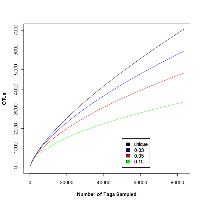
The largest sample in the Sogin data set was FS396. Originally represented by 17,666 sequences, the updated data set contains 83,399 sequences. This data set was used to generate rarefaction curves in Fig. 2 of the Sogin study. We did not observe any differences between the OTUs that were calculated for the unique, 0.01, and 0.02 OTU definitions. As mentioned above, this is probably due to muscle doing a poor job of maintaining positional homology within the alignment. Regardless, the following rarefaction.single command will generate the rarefaction curve data with updates every 5,000 sequences:
mothur > rarefaction.single(freq=5000)
To plot the data (shown on the right) we use R. The following commands will generate a set of rarefaction curves:
data<-read.table(file="sogin.unique.filter.fn.FS396.rarefaction", header=T)
plot(x=data$numsampled, y=data$unique, xlab="Number of Tags Sampled",ylab="OTUs", type="l", col="black", font.lab=3)
points(x=data$numsampled, y=data$X0.03, type="l", col="blue")
points(x=data$numsampled, y=data$X0.05, type="l", col="red")
points(x=data$numsampled, y=data$X0.10, type="l", col="green")
legend(x=50000, y=1500, c("unique", "0.03", "0.05", "0.10"), c("black", "blue", "red", "green"))
Clearly, regardless of the differences in methods and increased number of sequences, the story remains: a lot more sequences are needed to fully sample the community. This was basically as far as Sogin’s group took their OTU-based analysis.
Multi-sample rarefaction
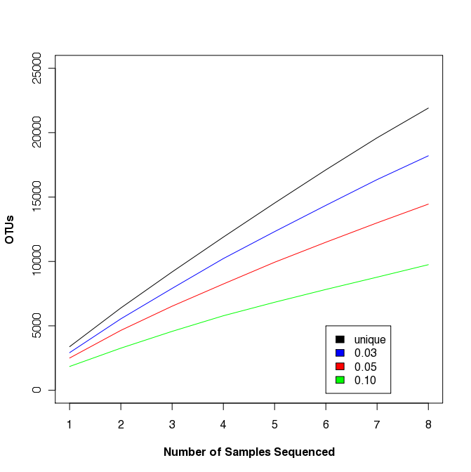 Traditional ecology studies will rarefy across samples, not sequences.
This is possible in mothur using the
rarefaction.shared command.
Traditional ecology studies will rarefy across samples, not sequences.
This is possible in mothur using the
rarefaction.shared command.
mothur > read.otu(shared=sogin.unique.filter.fn.shared)
mothur > rarefaction.shared()
Similar to the R commands described above, we can generate the rarefaction curve shown at the right. This study is somewhat artificial because the samples weren’t taken from the same site or at even spatial increments; however, you should be able to see that such curves could be fit to a power law model to assess biogeography or to obtain a more robust estimate of community richness.
Multi-community visualization tools
Venn diagrams
mothur gives the ability to visualize data using a number of different methods. First, we will generate a venn diagram describing the overlap between samples FS312 and FS396 based on the observed richness and the Chao1 estimators using the venn command. These samples were the most deeply sequenced samples and are from diffuse flows at the Bag City and Marker 52 sites, respectively, in the Axial Seamount, Juan de Fuca Ridge.
mothur > venn(calc=sharedsobs-sharedchao, groups=FS312-FS396, label=0.10)
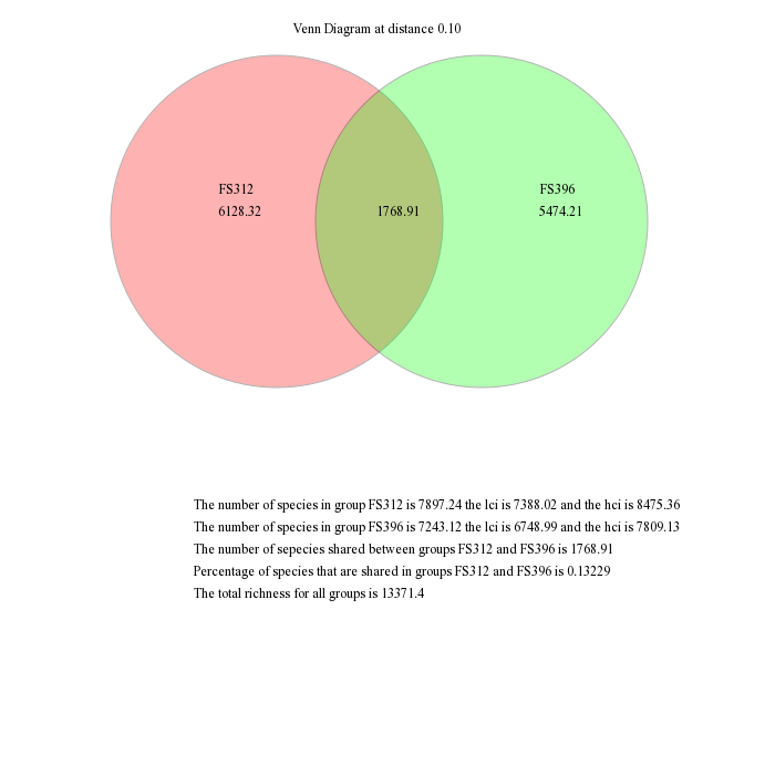
These are the raw output from mothur, which you would probably modify for publication in a program such as Adobe Illustrator. For example, you might like to scale the circles to be proportional to the richness the represent and remove the descriptive text.
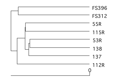
Dendrograms
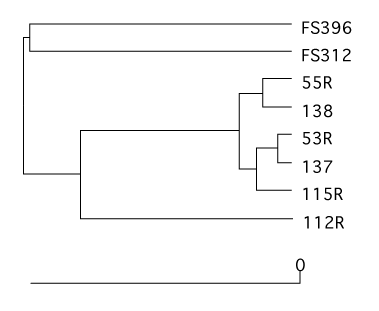
Using a number of similarity calculators you can generate dendrograms to relate the similarity in community membership and structure with the tree.shared command. To generate dendrograms based on membership we used the jest calculator, which uses the Chao estimator to predict the individual and shared richness values and we used the Yue & Clayton similarity value, θ~YC~.
mothur > tree.shared(calc=jest-thetayc)
This will generate two newick-formatted tree files - sogin.unique.filter.fn.thetayc.0.10.tre and sogin.unique.filter.fn.jest.0.10.tre. Using FigTree, these dendrograms can be displayed and exported as SVG image files. Again, these SVG files can be edited in a program like Adobe Illustrator. Here we present the dendrograms as exported from TreeViewX.
Heatmap
Finally, we’ll present the relative abundance of the OTUs found across all 8 communities for an 0.10 OTU definition. Because these data typically follow a highly skewed distribution, we will scale the relative abundance between red and black using a log-transformation using the heatmap.bin command. Missing data are shown as white blocks.
mothur > heatmap.bin(scale=log10)
This is clearly a lot of data! The scale bar is at the bottom of the heatmap and should be resized to be legible in Adobe Illustrator.
Conclusion
This demonstration hopefully gives a sense of the power, flexibility, and speed of mothur. If these commands were entered as a batch file, it would require less than 2 hrs to run on my laptop